I'm tickled pink to announce the release of mcradds (version 1.0.1) helps with designing, analyzing and visualization in In Vitro Diagnostic trials.
You can install it from CRAN with:
install.packages("mcradds")or you can install the development version directly from GitHub with:
if (!require("devtools")) {
  install.packages("devtools")
}
devtools::install_github("kaigu1990/mcradds")
This blog post will introduce you to package and desirability functions. Let's start loading this package.
library(mcradds)The mcradds R package is a complement to mcr package and it offers common and solid functions for designing, analyzing, and visualizing in In Vitro Diagnostic (IVD) trials. In my work experience as a statistician for diagnostic trials at Roche Diagnostic, mcr package is an internally built tool for analyzing regression and other relevant methodologies that are also widely used in the IVD industry community.
However, the mcr package focuses on method comparison trials and does not include additional common diagnostic methods but that have been provided in the mcradds. It is intuitive and easy to use. So you can perform statistical analysis and graphics in different IVD trials utilizing the analytical functions.
- Estimate the sample size for trials, following NMPA guidelines.
- Evaluate diagnostic accuracy with/without reference, following CLSI EP12-A2.
- Perform regression method analysis and plots, following CLSI EP09-A3.
- Perform bland-Altman analysis and plots, following CLSI EP09-A3.
- Detect outliers with 4E method from CLSI EP09-A2 and ESD from CLSI EP09-A3.
- Estimate bias in medical decision level, following CLSI EP09-A3.
- Perform Pearson and Spearman correlation analysis, adding hypothesis test and confidence interval.
- Evaluate Reference Range/Interval, following CLSI EP28-A3 and NMPA guidelines.
- Add paired ROC/AUC test for superiority and non-inferiority trials, following CLSI EP05-A3/EP15-A3.
- Perform reproducibility analysis (reader precision) for immunohistochemical assays, following CLSI I/LA28-A2 and NMPA guidelines.
- Evaluate precision of quantitative measurements, following CLSI EP05-A3.
Please be noted that these functions and methods have not been validated and QC'ed, so I cannot guarantee that all of them are entirely proper and error-free. But I always strive to compare the results to those of other resources in order to obtain a consistent result for them. And because some of them were utilized in my past usual work process, I believe the quality of this package is temporarily sufficient to use.
Let's demonstrate that by looking at a few of examples. More detailed usages can be found in Get started page
Suppose that we have a new diagnostic assay with the expected sensitivity criteria of 0.9, and the clinical acceptable criteria is 0.85. If we conduct a two-sided normal Z-test at a significance level of α = 0.05 and achieve a power of 80%, what should the total sample size be?
The result from sample size function is:
size_one_prop(p1 = 0.9, p0 = 0.85, alpha = 0.05, power = 0.8)
#>
#>  Sample size determination for one Proportion
#>
#>  Call: size_one_prop(p1 = 0.9, p0 = 0.85, alpha = 0.05, power = 0.8)
#>
#>    optimal sample size: n = 363
#>
#>    p1:0.9 p0:0.85 alpha:0.05 power:0.8 alternative:two.sided
Suppose that you have a wide structure of data like qualData that contains the qualitative measurements of the candidate (your own product) and comparative (reference product) assays. In this scenario, if you’re interested in how to create a 2x2 contingency table, the diagTab() function is a good solution.
data("qualData")
tb <- qualData %>%
  diagTab(
    formula = ~ CandidateN + ComparativeN,
    levels = c(1, 0)
  )
tb
#> Contingency Table:
#>
#> levels: 1 0
#>           ComparativeN
#> CandidateN   1   0
#>          1 122   8
#>          0  16  54
However, there are different formula settings when the data structure is long.
dummy <- data.frame(
  id = c("1001", "1001", "1002", "1002", "1003", "1003"),
  value = c(1, 0, 0, 0, 1, 1),
  type = c("Test", "Ref", "Test", "Ref", "Test", "Ref")
) %>%
  diagTab(
    formula = type ~ value,
    bysort = "id",
    dimname = c("Test", "Ref"),
    levels = c(1, 0)
  )
dummy
#> Contingency Table:
#>
#> levels: 1 0
#>     Ref
#> Test 1 0
#>    1 1 1
#>    0 0 1
And then you can use the getAccuracy() method to compute the diagnostic performance based on the table above.
# Default method is Wilson score, and digit is 4.
tb %>% getAccuracy(ref = "r")
#>         EST LowerCI UpperCI
#> sens 0.8841  0.8200  0.9274
#> spec 0.8710  0.7655  0.9331
#> ppv  0.9385  0.8833  0.9685
#> npv  0.7714  0.6605  0.8541
#> plr  6.8514  3.5785 13.1181
#> nlr  0.1331  0.0832  0.2131
If you want to estimate the reader precision between different readers, reads, or sites, use the APA, ANA and OPA as the primary endpoint in the PDL1 assay trials. Let’s see an example of precision between readers.
data("PDL1RP")
reader <- PDL1RP$btw_reader
tb1 <- reader %>%
diagTab(
formula = Reader ~ Value,
bysort = "Sample",
levels = c("Positive", "Negative"),
rep = TRUE,
across = "Site"
)
getAccuracy(tb1, ref = "bnr", rng.seed = 12306)
#> EST LowerCI UpperCI
#> apa 0.9479 0.9260 0.9686
#> ana 0.9540 0.9342 0.9730
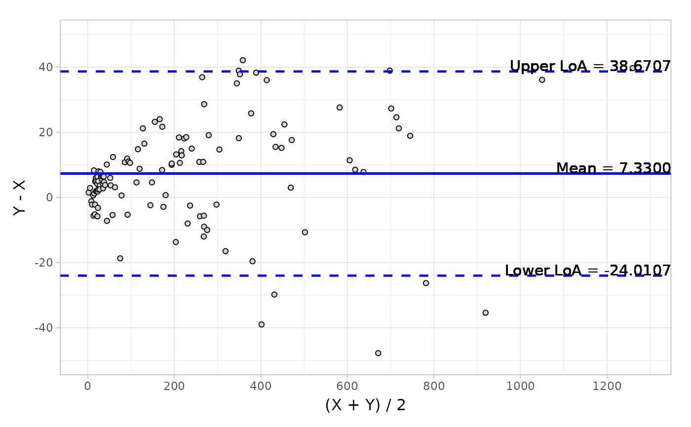
#> opa 0.9511 0.9311 0.9711Suppose that in another scenario, you have a wide structure of quantitative data like platelet and would like to do the Bland-Altman analysis to obtain a series of descriptive statistics including, mean, median, Q1, Q3, min, max and other estimations like CI (confidence interval of mean) and LoA (Limit of Agreement).
data("platelet")
# Default difference type
blandAltman(
  x = platelet$Comparative, y = platelet$Candidate,
  type1 = 3, type2 = 5
)
#>  Call: blandAltman(x = platelet$Comparative, y = platelet$Candidate,
#>     type1 = 3, type2 = 5)
#>
#>   Absolute difference type:  Y-X
#>   Relative difference type:  (Y-X)/(0.5*(X+Y))
#>
#>                             Absolute.difference Relative.difference
#> N                                           120                 120
#> Mean (SD)                        7.330 (15.990)      0.064 ( 0.145)
#> Median                                    6.350               0.055
#> Q1, Q3                         ( 0.150, 15.750)    ( 0.001,  0.118)
#> Min, Max                      (-47.800, 42.100)    (-0.412,  0.667)
#> Limit of Agreement            (-24.011, 38.671)    (-0.220,  0.347)
#> Confidence Interval of Mean    ( 4.469, 10.191)    ( 0.038,  0.089)
And the visualization of Bland-Altman can be easily conducted by the autoplot method.
object <- blandAltman(x = platelet$Comparative, y = platelet$Candidate)

# Absolute difference plot
autoplot(object, type = "absolute")
Here is a plot of the data.
Based on the output from Bland-Altman, you can also detect the potential outliers using the getOutlier() method.
# ESD approach
ba <- blandAltman(x = platelet$Comparative, y = platelet$Candidate)
out <- getOutlier(ba, method = "ESD", difference = "rel")
out$stat
#> i Mean SD x Obs ESDi Lambda Outlier
#> 1 1 0.06356753 0.1447540 0.6666667 1 4.166372 3.445148 TRUE
#> 2 2 0.05849947 0.1342496 0.5783972 4 3.872621 3.442394 TRUE
#> 3 3 0.05409356 0.1258857 0.5321101 2 3.797226 3.439611 TRUE
#> 4 4 0.05000794 0.1183096 -0.4117647 10 3.903086 3.436800 TRUE
#> 5 5 0.05398874 0.1106738 -0.3132530 14 3.318236 3.433961 FALSE
#> 6 6 0.05718215 0.1056542 -0.2566372 23 2.970250 3.431092 FALSE
out$outmat
#> sid x y
#> 1 1 1.5 3.0
#> 2 2 4.0 6.9
#> 3 4 10.2 18.5
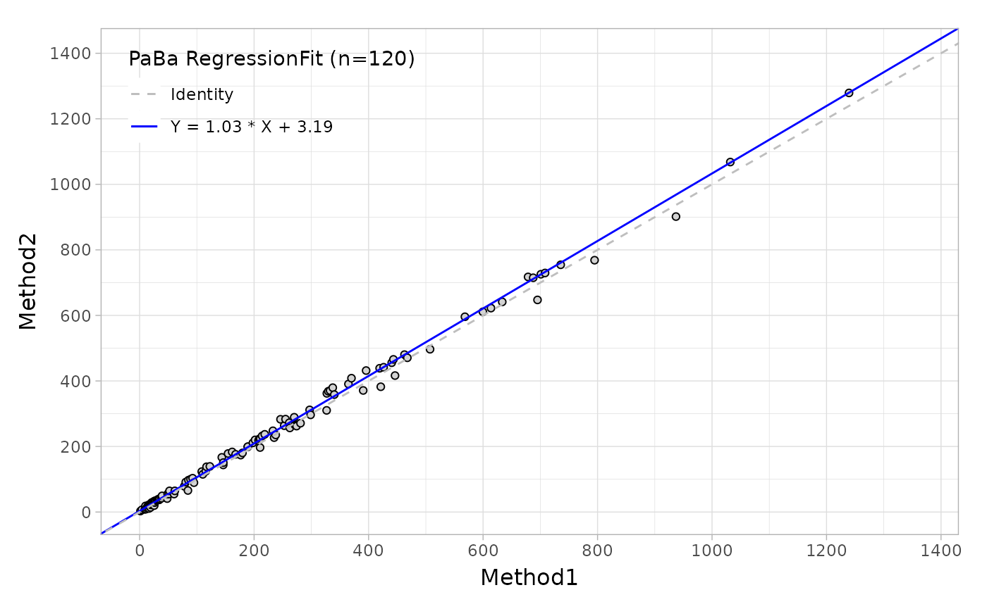
#> 4 10 16.4 10.8Suppose that you would like to evaluate the regression agreement between two assays with 'Deming' method, you can use the mcreg, this main function is wrapped from mcr package.
# Deming regression
fit <- mcreg(
  x = platelet$Comparative, y = platelet$Candidate,
  error.ratio = 1, method.reg = "Deming", method.ci = "jackknife"
)
Like the Bland-Altman plot, as well as in regression plot, the autoplot function can provide the scatter plot with a fitted line as shown below.
Based on this regression analysis, you can also estimate the bias at one or more medical decision levels.
# absolute bias.
calcBias(fit, x.levels = c(30))
#>    Level     Bias       SE      LCI      UCI
#> X1    30 4.724429 1.378232 1.995155 7.453704

# proportional bias.
calcBias(fit, x.levels = c(30), type = "proportional")
#>    Level Prop.bias(%)       SE      LCI      UCI
#> X1    30      15.7481 4.594106 6.650517 24.84568
Suppose that you have a target population data, and would like to compute the 95% reference interval (RI) with non-paramtric method.
data("calcium")
refInterval(x = calcium$Value, RI_method = "nonparametric", CI_method = "nonparametric")
#>
#>  Reference Interval Method: nonparametric, Confidence Interval Method: nonparametric
#>
#>  Call: refInterval(x = calcium$Value, RI_method = "nonparametric", CI_method = "nonparametric")
#>
#>   N = 240
#>   Outliers: NULL
#>   Reference Interval: 9.10, 10.30
#>   RefLower Confidence Interval: 8.9000, 9.2000
#>   Refupper Confidence Interval: 10.3000, 10.4000
Suppose that you want to see if the OxLDL assay is superior to the LDL assay through comparing two AUC of paired two-sample diagnostic assays using the standardized difference method when the margin is equal to 0.1. In this case, the null hypothesis is that the difference is less than 0.1.
data("ldlroc")
# H0 : Superiority margin <= 0.1:
aucTest(
  x = ldlroc$LDL, y = ldlroc$OxLDL, response = ldlroc$Diagnosis,
  method = "superiority", h0 = 0.1
)
#> Setting levels: control = 0, case = 1
#> Setting direction: controls < cases
#>
#> The hypothesis for testing superiority based on Paired ROC curve
#>
#>  Test assay:
#>   Area under the curve: 0.7995
#>   Standard Error(SE): 0.0620
#>   95% Confidence Interval(CI): 0.6781-0.9210 (DeLong)
#>
#>  Reference/standard assay:
#>   Area under the curve: 0.5617
#>   Standard Error(SE): 0.0836
#>   95% Confidence Interval(CI): 0.3979-0.7255 (DeLong)
#>
#>  Comparison of Paired AUC:
#>   Alternative hypothesis: the difference in AUC is superiority to 0.1
#>   Difference of AUC: 0.2378
#>   Standard Error(SE): 0.0790
#>   95% Confidence Interval(CI): 0.0829-0.3927 (standardized differenec method)
#>   Z: 1.7436
#>   Pvalue: 0.04061
Suppose that you feel like to do the hypothesis test of H0=0.7 not H0=0 with pearson and spearman correlation analysis, the pearsonTest() and spearmanTest() would be helpful.
# Pearson hypothesis test
x <- c(44.4, 45.9, 41.9, 53.3, 44.7, 44.1, 50.7, 45.2, 60.1)
y <- c(2.6, 3.1, 2.5, 5.0, 3.6, 4.0, 5.2, 2.8, 3.8)
pearsonTest(x, y, h0 = 0.5, alternative = "greater")
#> $stat
#>        cor    lowerci    upperci          Z       pval
#>  0.5711816 -0.1497426  0.8955795  0.2448722  0.4032777
#>
#> $method
#> [1] "Pearson's correlation"
#>
#> $conf.level
#> [1] 0.95

# Spearman hypothesis test
x <- c(44.4, 45.9, 41.9, 53.3, 44.7, 44.1, 50.7, 45.2, 60.1)
y <- c(2.6, 3.1, 2.5, 5.0, 3.6, 4.0, 5.2, 2.8, 3.8)
spearmanTest(x, y, h0 = 0.5, alternative = "greater")
#> $stat
#>        cor    lowerci    upperci          Z       pval
#>  0.6000000 -0.1478261  0.9656153  0.3243526  0.3728355
#>
#> $method
#> [1] "Spearman's correlation"
#>
#> $conf.level
#> [1] 0.95
That's it! That's the mcradds package. More details can be found in the Introduction to mcradds vignette.