<?xml version="1.0" encoding="utf-8"?>
<feed xmlns="http://www.w3.org/2005/Atom">
  <title>KeepNotes blog</title>
  
  <subtitle>Stay hungry, Stay Foolish.</subtitle>
  <link href="/atom.xml" rel="self"/>
  
  <link href="http://www.bioinfo-scrounger.com/"/>
  <updated>2024-09-19T02:08:37.496Z</updated>
  <id>http://www.bioinfo-scrounger.com/</id>
  
  <author>
    <name>Kai</name>
    
  </author>
  
  <generator uri="https://hexo.io/">Hexo</generator>
  
  <entry>
    <title>Miettinen-Nurminen (MN) Test in R and SAS</title>
    <link href="http://www.bioinfo-scrounger.com/archives/mn_test/"/>
    <id>http://www.bioinfo-scrounger.com/archives/mn_test/</id>
    <published>2024-09-19T02:03:21.000Z</published>
    <updated>2024-09-19T02:08:37.496Z</updated>
    
    <content type="html"><![CDATA[<p>Miettinen-Nurminen (MN) method has increasingly been requested by regulatory agencies, rather than the traditional Wald method that is based on the asymptotic normal distribution. This is particularly relevant for non-inferiority trials where it's appropriate for the variance to be estimated under the null hypothesis. <a href="https://communities.sas.com/t5/SAS-Product-Suggestions/Calculate-MN-Test-Statistics-within-PROC-FREQ/idi-p/933198" target="_blank" rel="noopener">Calculate MN Test Statistics within PROC FREQ</a>.</p><a id="more"></a><p>The formula for compute the MN test statistic can be found in many articles, such as a paper in lexjansen <a href="https://www.lexjansen.com/wuss/2016/127_Final_Paper_PDF.pdf" target="_blank" rel="noopener">Constructing Confidence Intervals for the Differences of Binomial Proportions in SAS</a>.</p><figure><img src="https://www.bioinfo-scrounger.com/data/photo/MN_formula.png" alt="" /><figcaption>MN_formula</figcaption></figure><p>As can be seen from the above description, if we would like to get the CI of M&amp;N method, we should compute the root of the maximum likelihood estimations with the closed-form solution provided by M&amp;N. Referring to the following method from <a href="https://merck.github.io/metalite.ae/articles/rate-compare.html" target="_blank" rel="noopener">metalite.ae rate-compare vignettes</a>, we can create an equation <code>p2 - p1 = delta</code> and the chi-square statistic to find out the root.</p><figure><img src="https://www.bioinfo-scrounger.com/data/photo/MN_formula2.png" alt="" /><figcaption>MN_formula2</figcaption></figure><p>As can be seen from the above explanation, if we would like to get the confidence interval (CI) of M&amp;N method, we should compute the root of the maximum likelihood estimations with the closed-form solution provided by M&amp;N. Referring to the following method, we can construct an equation to find out the root from the chi-square distribution with 1 degree of freedom. So I roughly understand that the delta can be regarded as the CI when the equation of <code>p1 - p2 - delta</code> divided by variance is equivalent to the chi-square statistic. Therefore, I create a function so that I can obtain the root using a solving process.</p><pre><code>mn_root &lt;- function(delta, alpha = 0.05) {  diff &lt;- p1 - p2 - delta  theta &lt;- n2 / n1  a &lt;- 1 + theta  b &lt;- -(1 + theta + p1 + theta * p2 + delta * (theta + 2))  c &lt;- delta^2 + delta * (2 * p1 + theta + 1) + p1 + theta * p2  d &lt;- -p1 * delta * (1 + delta)  v &lt;- b^3 / (27 * a^3) - b * c / (6 * a^2) + d / (a * 2)  # here should be &#39;-&#39; instead of &#39;+&#39; inside the square root.  u &lt;- ifelse(v &gt; 0, 1, -1) * sqrt(b^2 / (9 * a^2) - c / (a * 3))  w &lt;- (pi + acos(v / u^3)) / 3  p1d &lt;- 2 * u * cos(w) - b / (a * 3)  p2d &lt;- p1d - delta  # n &lt;- n1 + n2  var &lt;- (p1d * (1 - p1d) / n1 + p2d * (1 - p2d) / n2) * (n1 + n2) / (n1 + n2 - 1)  chisq &lt;- diff^2 / var  return(chisq - qchisq(1 - alpha, 1))}</code></pre><p>Now I also create an example data as shown below to compute the risk difference (RD) of response rate between two treatments.</p><pre><code>library(tidyverse)ana &lt;- data.frame(  treatment = factor(c(rep(2, 100), rep(1, 100)), level = c(2, 1)),  response  = c(rep(0, 80), rep(1, 20), rep(0, 40), rep(1, 60)),  stratum   = c(rep(1:4, 12), 1, 3, 3, 1, rep(1:4, 12), rep(1:4, 25)))</code></pre><p>By this example data, I can know the sample size and response rate for each treatment group. And then in order to obtain the root, someone will use the bisection method but I feel that we can just use the <code>uniroot()</code> to solve the single root, or <code>rootSolve::uniroot.all()</code> to get multiple roots.</p><pre><code>p1 &lt;- 0.6p2 &lt;- 0.2n1 &lt;- 100n2 &lt;- 100rootSolve::uniroot.all(mn_root, interval = c(-0.999, 0.999), n = 100, tol = 1e-6)## [1] 0.2696618 0.5165744    </code></pre><p>Then I use the <code>metalite.ae::rate_compare()</code> to check the result from the above self-defined function. Both of the upper and lower values of CI are consistent.</p><pre><code>metalite.ae::rate_compare(response ~ treatment, data = ana)##   est  z_score            p    lower     upper## 1 0.4 5.759051 4.229411e-09 0.269662 0.5165743</code></pre><hr /><p>According to the stratified M&amp;N test, I will just talk about it briefly here. If you would like to use the Miettinen-Nurminen stratified method as described in the 1985 paper by SAS, unfortunately the current SAS version cannot support it yet. Although I can use <code>COMMONRISKDIFF(CL=score)</code> to compute the CI of risk difference, the results are not the MN 1985 method that is referred to as Agresti Score at the summary level. More discussions can be found in <a href="https://communities.sas.com/t5/SASware-Ballot-Ideas/Confidence-limits-using-the-Miettinen-Nurminen-stratified-method/idi-p/829317" target="_blank" rel="noopener">Confidence limits using the Miettinen-Nurminen stratified method as described in the 1985 paper</a>, and <a href="https://communities.sas.com/t5/SAS-Product-Suggestions/Calculate-MN-Test-Statistics-within-PROC-FREQ/idi-p/933198" target="_blank" rel="noopener">Calculate MN Test Statistics within PROC FREQ</a>.</p><p>The basic SAS and R codes for example data used to compute the unstratified and stratified Miettinen and Nurminen test are provided below for reference. It should be emphasized that the results of stratified M&amp;N results are not consistent.</p><p>R code:</p><pre><code># Unstratified M&amp;N testmetalite.ae::rate_compare(  formula = response ~ treatment, data = ana)# Stratified M&amp;N testmetalite.ae::rate_compare(  formula = response ~ treatment, data = ana,  strata = stratum, weight = &quot;ss&quot;)##         est  z_score            p     lower     upper## 1 0.3998397 5.712797 5.556727e-09 0.2684383 0.5172779</code></pre><p>SAS code:</p><pre><code>data ana;    input id trtpn stratum response count;    datalines;1  0 1 0 212  0 1 1 53  0 2 0 194  0 2 1 55  0 3 0 216  0 3 1 57  0 4 0 198  0 4 1 59  1 1 0 1010 1 1 1 1511 1 2 0 1012 1 2 1 1513 1 3 0 1014 1 3 1 1515 1 4 0 1016 1 4 1 15;run;ods listing close;proc freq data=ana;    weight count/zeros;    tables trtpn*response/ riskdiff(CL=mn) alpha=0.05;     ods output PdiffCLs=respdiff;run;ods listing;ods listing close;proc freq data=ana;    weight count/zeros;    tables stratum*trtpn*response/ riskdiff(CL=mn)         COMMONRISKDIFF(CL=(score) test=(score)) alpha=0.05;     ods output PdiffCLs=respdiff CommonPdiff=compdiff;run;ods listing;</code></pre><figure><img src="https://www.bioinfo-scrounger.com/data/photo/MN_formula_SAS.png" alt="" /><figcaption>MN_formula_SAS</figcaption></figure>]]></content>
    
    <summary type="html">
    
      &lt;p&gt;Miettinen-Nurminen (MN) method has increasingly been requested by regulatory agencies, rather than the traditional Wald method that is based on the asymptotic normal distribution. This is particularly relevant for non-inferiority trials where it&#39;s appropriate for the variance to be estimated under the null hypothesis. &lt;a href=&quot;https://communities.sas.com/t5/SAS-Product-Suggestions/Calculate-MN-Test-Statistics-within-PROC-FREQ/idi-p/933198&quot; target=&quot;_blank&quot; rel=&quot;noopener&quot;&gt;Calculate MN Test Statistics within PROC FREQ&lt;/a&gt;.&lt;/p&gt;
    
    </summary>
    
    
      <category term="Biometrics" scheme="http://www.bioinfo-scrounger.com/categories/Biometrics/"/>
    
      <category term="BiomedicalStats" scheme="http://www.bioinfo-scrounger.com/categories/Biometrics/BiomedicalStats/"/>
    
    
      <category term="Statistics" scheme="http://www.bioinfo-scrounger.com/tags/Statistics/"/>
    
  </entry>
  
  <entry>
    <title>Learning Bisection Method</title>
    <link href="http://www.bioinfo-scrounger.com/archives/bisection/"/>
    <id>http://www.bioinfo-scrounger.com/archives/bisection/</id>
    <published>2024-07-03T12:09:23.000Z</published>
    <updated>2024-07-03T12:14:17.442Z</updated>
    
    <content type="html"><![CDATA[<p>When I learned the Miettinen and Nurminen Test algorithm from the <code>rate-compare</code> article (<a href="https://cran.r-project.org/web/packages/metalite.ae/vignettes/rate-compare.html" target="_blank" rel="noopener">Unstratified and Stratified Miettinen and Nurminen Test</a>), I found that its CI is given by the roots of an equation. In order to reproduce its algorithm, I'd like to learn more about the Bisection method first.</p><a id="more"></a><p>The bisection method is an approach to finding the root of a continuous function on an interval. Its principle can be shown below (referring from <a href="https://rpubs.com/aaronsc32/bisection-method-r" target="_blank" rel="noopener">https://rpubs.com/aaronsc32/bisection-method-r</a>).</p><blockquote><p>The method takes advantage of a corollary of the <a href="https://en.wikipedia.org/wiki/Intermediate_value_theorem" target="_blank" rel="noopener">intermediate value theorem</a> called Bolzano's theorem which states that if the values of f(a) and f(b) have opposite signs, the interval must contain at least one root. The iteration steps of the bisection method are relatively straightforward, however; convergence towards a solution is slow compared to other root-finding methods.</p></blockquote><p>Thus the algorithm can be divided into the following steps. - Calculate the minpoint <code>m=(a+b)/2</code> based on the interval with the lower bound <code>a</code> and higher bound <code>b</code>. - Get the value of function <code>f</code> at midpoint. If <code>f(a)</code> and <code>f(m)</code> have opposite signs, then <code>b</code> point is replaced by the computed midpoint, or if <code>f(b)</code> and <code>f(m)</code> have opposite signs, <code>a</code> is replaced by midpoint. This step ensures the root of function can be kept within the new interval. - Iterate over the above steps 1-2 until the difference between <code>a</code> and <code>b</code> is small enough or the defined iterating number is reached, at which midpoint <code>m</code> is the root.</p><p>According to the above steps, we can write a function to implement the bisection method in R. Assume we have the following function <code>f</code> to be solved.</p><pre><code>f &lt;- function(x) cos(x)^4 - 4*cos(x)^3 + 8*cos(x)^2 - 5*cos(x) + 1/2</code></pre><p>Then we create a function with bisection algorithm and find the root.</p><pre><code>bisect_func &lt;- function(f, a, b, tol = 1e-5, n = 100) {  i &lt;- 1  while (i &lt;= n) {    m &lt;- (a + b) / 2    if (abs(b - a) &lt; tol | f(m) == 0) {      break    }        if (f(a) * f(m) &lt;0) {      b &lt;- m    } else if (f(b) * f(m) &lt; 0) {      a &lt;- m    } else {      stop(&quot;f(a) and f(b) must have opposite sign.&quot;)    }        i &lt;- i + 1    if (i &gt; n) {      warning(&quot;The max iterations reached, maybe the lower and upper bound should be changed and try again.&quot;)    }  }  root &lt;- (a + b) / 2  return(root)}bisect_func(f, 0, 2, tol = 0.001)[1] 0.6293945</code></pre><p>And the same outcome can be obtained from the mature function <code>cmna::bisection()</code>.</p><pre><code>cmna::bisection(f, 0, 2)[1] 0.6293945</code></pre><p>Actually this <code>f</code> function should have two roots, but the <code>bisect_func()</code> or <code>cmna::bisection()</code> functions trend to have the root on the lower bound side. In this case, we must either run the bisection function multiple times for different intervals, or use another function able to finding multiple roots.</p><pre><code># two roots in (0,1) and (1,2)bisect_func(f, 0, 1, tol = 0.001)[1] 0.6293945bisect_func(f, 1, 2, tol = 0.001)[1] 1.447754# using uniroot.all() functionrootSolve::uniroot.all(f, c(0, 2), n = 100)[1] 0.6293342 1.4480258</code></pre><hr /><p>Above is my brief summary and hope it can be useful. And in the following post I will learn how to use bisection method or uniroot function to solve in the Miettinen-Nurminen (Score) Confidence Limits.</p><h4 id="reference">Reference</h4><p><a href="https://rpubs.com/aaronsc32/bisection-method-r" target="_blank" rel="noopener">Bisection Method</a><br /><a href="https://www.r-bloggers.com/2015/10/finding-multiple-roots-of-univariate-functions-in-r/" target="_blank" rel="noopener">Finding multiple roots of univariate functions in R</a></p>]]></content>
    
    <summary type="html">
    
      &lt;p&gt;When I learned the Miettinen and Nurminen Test algorithm from the &lt;code&gt;rate-compare&lt;/code&gt; article (&lt;a href=&quot;https://cran.r-project.org/web/packages/metalite.ae/vignettes/rate-compare.html&quot; target=&quot;_blank&quot; rel=&quot;noopener&quot;&gt;Unstratified and Stratified Miettinen and Nurminen Test&lt;/a&gt;), I found that its CI is given by the roots of an equation. In order to reproduce its algorithm, I&#39;d like to learn more about the Bisection method first.&lt;/p&gt;
    
    </summary>
    
    
      <category term="Biometrics" scheme="http://www.bioinfo-scrounger.com/categories/Biometrics/"/>
    
      <category term="BioStats" scheme="http://www.bioinfo-scrounger.com/categories/Biometrics/BioStats/"/>
    
    
      <category term="Statistics" scheme="http://www.bioinfo-scrounger.com/tags/Statistics/"/>
    
  </entry>
  
  <entry>
    <title>Shift Value for MCMC imputation in Tipping Point Analysis</title>
    <link href="http://www.bioinfo-scrounger.com/archives/mcmc_tpa/"/>
    <id>http://www.bioinfo-scrounger.com/archives/mcmc_tpa/</id>
    <published>2024-07-03T12:05:18.000Z</published>
    <updated>2024-07-03T12:14:18.306Z</updated>
    
    <content type="html"><![CDATA[<p>This is a continuation of the previous article, <a href="https://www.bioinfo-scrounger.com/archives/tpa_mi/">Tipping Point Analysis in Multiple Imputation Using SAS</a>. In the last post, we talked about the tipping point analysis in monotone imputation, but how to implement TPA in MCMC imputation since the <code>MNAR</code> statement can only support the shift adjustment in monotone and FCS.</p><a id="more"></a><p>Before that, let's have a look at the process of imputation and shift adjustment in the monotone method. By default, the missing values are imputed sequentially in the order specified in the VAR statement. For example, the following <code>MI</code> procedure uses the regression method to impute each variable by its previous variables, which means variable <code>week8</code> is imputed by effects from <code>basval</code> to <code>week6</code>, and variable <code>week6</code> is imputed by effects from <code>basval</code> to <code>week4</code>. The variable <code>basval</code> is not imputed since it is the leading variable in the <code>VAR</code> statement. And you can also specify difference imputation methods in monotone statement for each variable, more details can be found in the <a href="https://documentation.sas.com/doc/en/statug/15.2/statug_mi_syntax09.htm#statug.mi.monoregopt" target="_blank" rel="noopener">SAS documentation</a></p><pre><code>proc mi data=low1_wide seed=12306 nimpute=10 out=imp_mnar2;    class trt;    by trt;    var basval week1 week2 week4 week6 week8;    monotone reg;    mnar adjust (week8 / shift=-1 adjustobs=(trt=&#39;1&#39;));    mnar adjust (week8 / shift=1 adjustobs=(trt=&#39;2&#39;));run;</code></pre><p>According to above logic, I feel we can manually add shift values instead of <code>MNAR</code> statement in the MCMC imputation by following the steps.</p><ul><li>Assuming the missingness pattern is arbitary rather than monotone, the MCMC full-data imputation approach is selected.</li><li>Get the imputed datasets and find out where the missing data is in the original dataset, such as the location of the subject and visit.</li><li>Adjust the <code>week8</code> variable with the shift values, for each treatment (if needed).</li></ul><p>I have tested the logic by comparing the results of the <code>MNAR</code> statement against manual adjusting. That is identical, so use the SAS code as shown below for MCMC imputation.</p><pre><code>proc mi data=low1_wide seed=12306 nimpute=10 out=imp_mcmc;    mcmc impute=full niter=1000 nbiter=1000;    by trt;    var basval week1 week2 week4 week6 week8;run;proc sort; by patient _imputation_; run;proc sort data=low1_wide     out=low1_wide_w8(keep=patient week8 rename=(week8=w8));     by patient;run;data imp_mcmc_shift;    merge imp_mcmc low1_wide_w8;    by patient;    if missing(w8) then do;        if trt=&#39;1&#39; then week8=week8-1;        else if trt=&#39;2&#39; then week8=week8+1;    end;    drop w8;run;</code></pre><p>As for the FCS approach, if you want to get the exact shift value, this article (<a href="https://www.pharmasug.org/proceedings/2023/SD/PharmaSUG-2023-SD-069.pdf" target="_blank" rel="noopener">Application of Tipping Point Analysis in Clinical Trials using the Multiple Imputation Procedure in SAS</a>) would be helpful.</p>]]></content>
    
    <summary type="html">
    
      &lt;p&gt;This is a continuation of the previous article, &lt;a href=&quot;https://www.bioinfo-scrounger.com/archives/tpa_mi/&quot;&gt;Tipping Point Analysis in Multiple Imputation Using SAS&lt;/a&gt;. In the last post, we talked about the tipping point analysis in monotone imputation, but how to implement TPA in MCMC imputation since the &lt;code&gt;MNAR&lt;/code&gt; statement can only support the shift adjustment in monotone and FCS.&lt;/p&gt;
    
    </summary>
    
    
      <category term="Biometrics" scheme="http://www.bioinfo-scrounger.com/categories/Biometrics/"/>
    
      <category term="BiomedicalStats" scheme="http://www.bioinfo-scrounger.com/categories/Biometrics/BiomedicalStats/"/>
    
    
      <category term="Statistics" scheme="http://www.bioinfo-scrounger.com/tags/Statistics/"/>
    
  </entry>
  
  <entry>
    <title>Tipping Point Analysis in Multiple Imputation using SAS</title>
    <link href="http://www.bioinfo-scrounger.com/archives/tpa_mi/"/>
    <id>http://www.bioinfo-scrounger.com/archives/tpa_mi/</id>
    <published>2024-07-01T12:37:07.000Z</published>
    <updated>2024-07-01T12:38:53.462Z</updated>
    
    <content type="html"><![CDATA[<p>The tipping point analysis has been a useful sensitivity analysis for multiple imputation to assess the robustness of the deviations from the MCAR or MAR assumptions. It aims to find out how severe departures from MAR will overturn the conclusions from primary analysis. If the departures are considered unlikely, this can give strong evidence supporting the treatment effect found in the primary analysis under the MAR assumptions.</p><a id="more"></a><p>In some ways, tipping point analysis can be regarded as supplementary to multiple imputation, allowing us to explore the outcomes from different scenarios by applying the shift parameters, such as decreasing the treatment effect while increasing the control group effect. The end goal is to identify the point at which the primary analysis result with multiple imputation becomes non-significant.</p><hr /><p>The tipping point analysis can be easily implemented using SAS procedure <code>PROC MI</code> and the brief instructions can be found in <a href="https://documentation.sas.com/doc/en/statug/15.2/statug_mianalyze_examples13.htm" target="_blank" rel="noopener">Sensitivity Analysis with the Tipping-Point Approach</a> where it uses the <code>MONOTONE</code> statement to impute the missing data and the <code>MNAR</code> statement to adjust the imputed data by a range of specified shift parameters. Thus the analysis steps can be described as follows:</p><ul><li>If the missing pattern you detect is intermittent rather than monotone, you should fill in the missing data using MCMC statement so that the pattern can be transformed into monotone.</li><li>If the missing data has monotone pattern, impute it using <code>MONOTONE</code> or <code>FCS</code> method in <code>Proc MI</code> under the MAR assumptions. And specify the shift parameters in <code>MNAR</code> statement to adjust the imputed value for observations in any treatment group as needed.</li><li>Based on the imputed datasets from step 2, apply the pre-specified models to analyze each dataset and obtain the statistical results.</li><li>Combine all of the results from step 3 by Rubin's rule using <code>Proc MIANALYZE</code> and make statistical inferences.</li><li>Repeat steps 2-4 by adjusting the shift parameters to get a set of inference outcomes to identify the tipping point that overturns the conclusions from significant to non-significant.</li></ul><p>Here, let's look at the SAS code below. I will use the example missing dataset (<code>low1.sas7bdat</code>) from Mallinckrodt et al. (<a href="https://journals.sagepub.com/doi/pdf/10.1177/2168479013501310" target="_blank" rel="noopener" class="uri">https://journals.sagepub.com/doi/pdf/10.1177/2168479013501310</a>). And transform it to fit the follow-up analysis requirement.</p><pre><code>proc sort data=low1; by patient trt basval; run;proc transpose data=low1 out=low1_wide(drop=_name_) prefix=week;    by patient trt basval;    id week;    var change;run;</code></pre><p>As I have checked this dataset has a monotone missing pattern, so I don't need to go through step 1. But if you need or want to achieve that, try the code below. Please note that we have generated <code>nimpute=10</code> imputed datasets in this step, we just need to apply <code>nimpute=1</code> in the next monotone imputation and MNAR adjust steps.</p><pre><code>/* Step 1: Achieve Monotone Missing Data Pattern */proc sort data=low1_wide; by trt; run;proc mi data=low1_wide seed=12306 nimpute=10 out=imp_mono;    mcmc impute=monotone nbiter=1000 niter=1000;    by trt;    var basval week1 week2 week4 week6 week8;run;/* Step2: MAR imputation and MNAR adjustation at week 8 visit for each group. */proc sort data=imp_mono; by _imputation_ trt; run;proc mi data=imp_mono seed=12306 nimpute=10 out=imp_mnar2;    class trt;    by _imputation_ trt;    var trt basval week1 week2 week4 week6 week8;    monotone reg;    mnar adjust (week8 / shift=-1 adjustobs=(trt=&#39;1&#39;));    mnar adjust (week8 / shift=1 adjustobs=(trt=&#39;2&#39;));run;</code></pre><p>Back to assuming the example dataset has a monotone pattern, we just jump into step 2. Here, I suppose the primary endpoint is the change from baseline at week 8. So the prior visits are imputed under the MAR assumption using <code>MONOTONE REG</code>, and the week 8 visit will have an additional <code>MNAR</code> process where the <code>trt=1</code> group is made better by adding a delta (<code>shift=-1</code>) while the <code>trt=2</code> group is made worse by a delta (<code>shift=1</code>) as the lower value implies the better treatment effect. I also want to impute the datasets separately for each treatment group, so I set the <code>BY</code> statement to <code>trt</code>.</p><pre><code>/* Step2: MAR imputation using MONOTONE */proc sort data=low1_wide; by trt; run;proc mi data=low1_wide seed=12306 nimpute=10 out=imp_mnar2;    class trt;    by trt;    var basval week1 week2 week4 week6 week8;    monotone reg;    mnar adjust (week8 / shift=-1 adjustobs=(trt=&#39;1&#39;));    mnar adjust (week8 / shift=1 adjustobs=(trt=&#39;2&#39;));run;</code></pre><p>From the SAS documentation, the <code>MNAR</code> statement is applicable only if it is used along with the <code>MONOTONE</code> and <code>FCS</code> statement. So why did I choose the former one here instead of the latter? Refer to this article (<a href="https://www.pharmasug.org/proceedings/2023/SD/PharmaSUG-2023-SD-069.pdf" target="_blank" rel="noopener">Application of Tipping Point Analysis in Clinical Trials using the Multiple Imputation Procedure in SAS</a>), it states that only <code>MONOTONE</code> can provide us with the exact shift value we specified in imputed values straightforwardly, whereas the <code>FCS</code> needs a bit trick processing although it has more advantages somewhere. P.S. I did check it, indeed as mentioned above.</p><p>Now we generate 10 imputed datasets with a single shift value, and then these complete datasets are analyzed using the ANCOVA model, and the results are combined using <code>Proc MIANALYZE</code>, which is a typical multiple imputation process. So we don't need to describe them as details, just put all of above steps into one macro so that we can get a set of results using different shift values.</p><pre><code>%macro mi_tpa(ind=, smin=, smax=, sinc=, out=);    /* Create a set of shift values */    %let ncase=%sysevalf((&amp;smax. - &amp;smin.) / &amp;sinc., ceil);        data &amp;out.;        set _null_;    run;        /* Looping implement each shift for monotone imputation */    %do i=0 %to &amp;ncase.;        %let k=%sysevalf(&amp;smin. + &amp;i. * &amp;sinc.);                proc sort data=&amp;ind.; by trt; run;        proc mi data=&amp;ind. seed=12306 nimpute=10 out=imp_mnar;            class trt;            by trt;            var basval week1 week2 week4 week6 week8;            monotone reg;            mnar adjust (week8 / shift=-&amp;k. adjustobs=(trt=&#39;1&#39;));            mnar adjust (week8 / shift=&amp;k. adjustobs=(trt=&#39;2&#39;));        run;        proc sort; by _imputation_; run;                /* Step 3: Implement ANCOVA model for each imputation*/        ods output lsmeans=lsm diffs=diff;         proc mixed data=imp_mnar;             by _imputation_;             class trt(ref=&#39;1&#39;);             model week8=basval trt /ddfm=kr;             lsmeans trt / cl pdiff diff;        run;        /* Step 4: Pooling model results */        ods output ParameterEstimates=combined_diff;         proc mianalyze data=diff;            by trt _trt;            modeleffects estimate;             stderr stderr;        run;                /* Output results */        data mnar;            set combined_diff;            shift=&amp;k.;        run;        data &amp;out.;            set &amp;out. mnar;        run;    %end;%mend;</code></pre><p>Here, we assume that the tipping point that reverses the conclusion is between 0 and 5. Thus I define the range from 0 to 5 with an interval of 0.5. The following code performs the <code>MNAR</code> adjustment with each of the shift values, like <code>0</code>, <code>0.5</code>, <code>1</code>,...,<code>4.5</code>, <code>5</code>.</p><pre><code>%mi_tpa(ind=low1_wide, smin=0, smax=5, sinc=0.5, out=tpa_rst);</code></pre><p>The output table can be shown below.</p><figure><img src="https://www.bioinfo-scrounger.com/data/photo/TPA_MNAR.png" alt="" /><figcaption>TPA_MNAR</figcaption></figure><p>Regarding each shift value, the smallest value where the p-value is no longer significant is identified as the tipping point (in the red box). The next question is whether the shift value is reasonable in clinical practice. If that is not reasonable or unlikely, it can provide strong support for out primary conclusion.</p><h4 id="reference">Reference</h4><p><a href="https://www.prometrika.com/thought-leadership/thought-leadership/tipping-point-analyses-in-missing-data-imputation/" target="_blank" rel="noopener">TIPPING POINT ANALYSES IN MISSING DATA IMPUTATION</a><br /><a href="https://www.pharmasug.org/proceedings/2023/SD/PharmaSUG-2023-SD-069.pdf" target="_blank" rel="noopener">Application of Tipping Point Analysis in Clinical Trials using the Multiple Imputation Procedure in SAS</a><br /><a href="https://classic.clinicaltrials.gov/ProvidedDocs/91/NCT03282591/SAP_001.pdf" target="_blank" rel="noopener">https://classic.clinicaltrials.gov/ProvidedDocs/91/NCT03282591/SAP_001.pdf</a><br /><a href="https://cdn.clinicaltrials.gov/large-docs/92/NCT03759392/SAP_001.pdf" target="_blank" rel="noopener">https://cdn.clinicaltrials.gov/large-docs/92/NCT03759392/SAP_001.pdf</a></p>]]></content>
    
    <summary type="html">
    
      &lt;p&gt;The tipping point analysis has been a useful sensitivity analysis for multiple imputation to assess the robustness of the deviations from the MCAR or MAR assumptions. It aims to find out how severe departures from MAR will overturn the conclusions from primary analysis. If the departures are considered unlikely, this can give strong evidence supporting the treatment effect found in the primary analysis under the MAR assumptions.&lt;/p&gt;
    
    </summary>
    
    
      <category term="Biometrics" scheme="http://www.bioinfo-scrounger.com/categories/Biometrics/"/>
    
      <category term="BiomedicalStats" scheme="http://www.bioinfo-scrounger.com/categories/Biometrics/BiomedicalStats/"/>
    
    
      <category term="Statistics" scheme="http://www.bioinfo-scrounger.com/tags/Statistics/"/>
    
  </entry>
  
  <entry>
    <title>Simply Understanding Log Rank Test</title>
    <link href="http://www.bioinfo-scrounger.com/archives/logrank-test/"/>
    <id>http://www.bioinfo-scrounger.com/archives/logrank-test/</id>
    <published>2024-06-26T15:23:23.000Z</published>
    <updated>2024-06-26T15:38:49.216Z</updated>
    
    <content type="html"><![CDATA[<p>The logrank test is the most commonly used statistical test in clinical trials to compare the survival distributions in different treatment groups. We usually just use the logrank results to test whether there is a difference between two survival curves. But what does this difference mean?</p><a id="more"></a><p>The main references are the two resources below.</p><ul><li><a href="https://datatab.net/tutorial/log-rank-test" target="_blank" rel="noopener">https://datatab.net/tutorial/log-rank-test</a></li><li><a href="https://web.stanford.edu/~lutian/coursepdf/unitweek3.pdf" target="_blank" rel="noopener">https://web.stanford.edu/~lutian/coursepdf/unitweek3.pdf</a></li></ul><p>First of all, the difference is a statistical concept, so we need a statistical hypothesis test to get the p-value in order to determine whether the difference is significant.</p><ul><li>Null hypothesis: The two treatment groups have identical survival distributions.</li><li>Alternative hypothesis: The two treatment groups have different survival distributions.</li></ul><p>Now the question turns to how to get the p-value. Before that we should obtain a test statistic that follows the a chi-squared distribution. Thus the question can be simplified to how to compute the test statistic, with details and equations available in the references above. Let's create an example data used to display the whole calculation process in R.</p><p>Suppose we have group 1 and group 2 including six time to event data. The table shows the survival time in <code>t</code> columns and the <code>evt</code> column tells us if an event occurred (<code>evt</code>=1) or the case censored (<code>evt</code>=0) in the corresponding time.</p><pre><code>d1 &lt;- data.frame(  t = c(3.1, 6.8, 9, 9, 11.3, 16.2),  evt = c(1, 0, 1, 1, 0, 1))d2 &lt;- data.frame(  t = c(8.7, 9, 10.1, 12.1, 18.7, 23.1),  evt = c(1, 1, 0, 0, 1, 0))</code></pre><p>Then we need to convert above datasets to unique survival times, summarize the number of events (<code>m</code> column) and consors (<code>q</code> column), and add one column to represent the risk number (<code>n</code> column) at each time. Then outer join two dataset using <code>t</code> variable and filter the invalid time as the time without events cannot offer any meaningful information for test statistic.</p><pre><code>dat1 &lt;- data.frame(  t = c(3.1, 6.8, 9, 11.3, 16.2),  m = c(1, 0, 2, 0, 1),  q = c(0, 1, 0, 1, 0),  n = c(6, 5, 4, 2, 1))dat2 &lt;- data.frame(  t = c(8.7, 9, 10.1, 12.1, 18.7, 23.1),  m = c(1, 1, 0, 0, 1, 0),  q = c(0, 0, 1, 1, 0, 1),  n = c(6, 5, 4, 3, 2, 1))dat &lt;- full_join(dat1, dat2, by = &quot;t&quot;, suffix = c(&quot;1&quot;, &quot;2&quot;)) %&gt;%  arrange(t) %&gt;%  filter(!(m1 %in% c(NA, 0) &amp; m2 %in% c(NA, 0))) %&gt;%  mutate(    across(contains(c(&quot;n&quot;)), \(x) ifelse(is.na(x), lead(x), x)),    across(contains(c(&quot;n1&quot;)), \(x) ifelse(row_number() == n(), lag(x) - lag(m1), x)),    across(contains(c(&quot;m&quot;, &quot;q&quot;)), \(x) replace_na(x, 0))  )##      t m1 q1 n1 m2 q2 n2## 1  3.1  1  0  6  0  0  6## 2  8.7  0  0  4  1  0  6## 3  9.0  2  0  4  1  0  5## 4 16.2  1  0  1  0  0  2## 5 18.7  0  0  0  1  0  2</code></pre><p>To get the statistic, we should firstly compute the so-called expected value (<code>e1</code> or <code>e2</code>), the difference (<code>me1</code> or <code>me2</code>) of the observed value (<code>m1</code> or <code>m2</code>) minus the expected values, and the variance (<code>v</code>).</p><pre><code>dat &lt;- dat %&gt;%  mutate(    e1 = n1 / (n1 + n2) * (m1 + m2),    e2 = n2 / (n1 + n2) * (m1 + m2),    me1 = m1 - e1,    me2 = m2 - e2,    v = (n1 * n2 * (m1 + m2) * (n1 + n2 - m1 - m2)) / ((n1 + n2)^2 * (n1 + n2 - 1))  )##      t m1 q1 n1 m2 q2 n2        e1        e2        me1        me2         v## 1  3.1  1  0  6  0  0  6 0.5000000 0.5000000  0.5000000 -0.5000000 0.2500000## 2  8.7  0  0  4  1  0  6 0.4000000 0.6000000 -0.4000000  0.4000000 0.2400000## 3  9.0  2  0  4  1  0  5 1.3333333 1.6666667  0.6666667 -0.6666667 0.5555556## 4 16.2  1  0  1  0  0  2 0.3333333 0.6666667  0.6666667 -0.6666667 0.2222222## 5 18.7  0  0  0  1  0  2 0.0000000 1.0000000  0.0000000  0.0000000 0.0000000</code></pre><p>Base on above computations, now we can simply calculate the test statistic, that is <code>1.6205</code> in our example. Then the p-value can be determined using the chi-squared distribution with one degree of freedom (number of groups minus 1).</p><pre><code>z &lt;- (sum(dat$me2))^2 / sum(dat$v)z## [1] 1.620508pchisq(z, df = 2 - 1, lower.tail = FALSE)## [1] 0.2030209</code></pre><p>Now that we should have a basic knowledge of <code>logrank</code>, and let us check with those found in the mature R package <code>survival</code>.</p><pre><code>data &lt;- bind_rows(  data.frame(    t = c(3.1, 6.8, 9, 9, 11.3, 16.2),    m = c(1, 0, 1, 1, 0, 1)  ),  data.frame(    t = c(8.7, 9, 10.1, 12.1, 18.7, 23.1),    m = c(1, 1, 0, 0, 1, 0)  )  , .id = &quot;grp&quot;)survdiff(formula = Surv(t, m==1) ~ grp, data = data)## Call:## survdiff(formula = Surv(t, m == 1) ~ grp, data = data)## ##       N Observed Expected (O-E)^2/E (O-E)^2/V## grp=1 6        4     2.57     0.800      1.62## grp=2 6        3     4.43     0.463      1.62## ##  Chisq= 1.6  on 1 degrees of freedom, p= 0.2 </code></pre><p>From above we can find the <code>Expected</code> column corresponds to the expected value we calculated, and the <code>Observed</code> column represents the observed value, and the <code>(O-E)^2/V</code> column represents the test statistic where the <code>V</code> is the variance of it. And both of them show the same chisq value and p-value.</p><p>For now perhaps you have a bette understanding of logrank test like me after going through the whole computation process.</p>]]></content>
    
    <summary type="html">
    
      &lt;p&gt;The logrank test is the most commonly used statistical test in clinical trials to compare the survival distributions in different treatment groups. We usually just use the logrank results to test whether there is a difference between two survival curves. But what does this difference mean?&lt;/p&gt;
    
    </summary>
    
    
      <category term="Biometrics" scheme="http://www.bioinfo-scrounger.com/categories/Biometrics/"/>
    
      <category term="BiomedicalStats" scheme="http://www.bioinfo-scrounger.com/categories/Biometrics/BiomedicalStats/"/>
    
    
      <category term="Statistics" scheme="http://www.bioinfo-scrounger.com/tags/Statistics/"/>
    
  </entry>
  
  <entry>
    <title>Quality control of SDTM using the sdtmchecks package</title>
    <link href="http://www.bioinfo-scrounger.com/archives/qc_sdtmchecks/"/>
    <id>http://www.bioinfo-scrounger.com/archives/qc_sdtmchecks/</id>
    <published>2024-06-19T13:09:02.000Z</published>
    <updated>2024-06-19T13:25:29.419Z</updated>
    
    <content type="html"><![CDATA[<p>如果想对SDTM有个快速全面的check，Pinnacle 21毫无疑问是首选，其能帮助我们对SDTM进行CDISC标准验证，发现data quality issue以及mapping不合理的之处。</p><a id="more"></a><p>若需要一些personalized check过程或者说company-specific check，那么<code>sdtmchecks</code> R包能提供一些非常有用的支持。就像<code>sdtmchecks</code>包介绍中所说的，其并不是想囊括所有SDTM check rules，也不是P21 data validation的复制替代品，其主要是想提供一个一般化且可操作并且有意义的data check。</p><hr /><blockquote><p><code>sdtmchecks</code>包囊括的方法和函数不多，应该说非常精简，但是都非常实用；这个也是我非常喜欢的方式，目标明确且提供适量的函数可供调用，学习曲线平缓。</p></blockquote><p>首先我们从github上安装其主分支下的版本</p><pre><code># install.packages(&quot;devtools&quot;)devtools::install_github(&quot;pharmaverse/sdtmchecks&quot;, ref=&quot;main&quot;)</code></pre><p>加载<code>sdtmchecks</code>包后我可以先初步浏览下其提供了多少内置的data check类型；当然也可用在网页端查阅，如：<a href="https://pharmaverse.github.io/sdtmchecks/articles/search_checks.html" target="_blank" rel="noopener">Search Data Check Functions</a>，其提供了非常详尽的 check details，以便我们理解最终报告中展示的内容。</p><pre><code>#Just type this insdtmchecksmeta</code></pre><p>接着我导入当前目录下所有SDTM数据集</p><pre><code>fn &lt;- list.files(  path = &quot;./SDTM&quot;,  pattern = &quot;sas7bdat&quot;, full.names = TRUE)for (file in fn) {  f &lt;- stringr::str_remove(basename(file), &quot;.sas7bdat&quot;)  assign(f, value = haven::read_sas(file))}</code></pre><p>然后可以选择run一个data check函数，函数名则可以从<code>sdtmchecksmeta</code>对象中获取，如<code>check_ae_aedecod(ae)</code>；或者run所有的check，如下所示：</p><pre><code>myreport &lt;- run_all_checks(  metads = sdtmchecksmeta,  priority = c(&quot;High&quot;, &quot;Medium&quot;, &quot;Low&quot;), # subset checks based on priority  type = c(&quot;ALL&quot;, &quot;ONC&quot;, &quot;PRO&quot;, &quot;OPHTH&quot;), # subset checks based category  verbose = TRUE)</code></pre><p>最后生成报告来审阅所有的data issues</p><pre><code>report_to_xlsx(res = myreport, outfile = &quot;sdtm_check_report.xlsx&quot;)</code></pre><p>但是不得不说，包内嵌的general check可能不太适用于我们的一些项目，这时需要比较精细的评估当前项目的sdtm需要哪些check模块，如：</p><pre><code># Subset to checks that should work OK for most datasetsmetads = sdtmchecksmeta %&gt;%  filter(check %in% c(&quot;check_ae_aedecod&quot;,                      &quot;check_ae_aetoxgr&quot;,                      &quot;check_ae_dup&quot;,                      &quot;check_cm_cmdecod&quot;,                      &quot;check_cm_missing_month&quot;,                      &quot;check_dm_age_missing&quot;,                      &quot;check_dm_usubjid_dup&quot;,                      &quot;check_dm_armcd&quot;                      ))myreport &lt;- run_all_checks(metads = metads, verbose = TRUE)</code></pre><p>必要的时候甚至可以自定义一些check，如：<a href="https://pharmaverse.github.io/sdtmchecks/articles/write_a_check.html" target="_blank" rel="noopener">Writing a New Check</a>。</p><p>以上均来自<code>sdtmchecks</code>包的文档，更多信息可查阅<a href="https://github.com/pharmaverse/sdtmchecks" target="_blank" rel="noopener">https://github.com/pharmaverse/sdtmchecks</a></p>]]></content>
    
    <summary type="html">
    
      &lt;p&gt;如果想对SDTM有个快速全面的check，Pinnacle 21毫无疑问是首选，其能帮助我们对SDTM进行CDISC标准验证，发现data quality issue以及mapping不合理的之处。&lt;/p&gt;
    
    </summary>
    
    
      <category term="Programming-Notes" scheme="http://www.bioinfo-scrounger.com/categories/Programming-Notes/"/>
    
      <category term="R" scheme="http://www.bioinfo-scrounger.com/categories/Programming-Notes/R/"/>
    
    
      <category term="R" scheme="http://www.bioinfo-scrounger.com/tags/R/"/>
    
  </entry>
  
  <entry>
    <title>Estimated LS-means from Multiple Imputation of mice using emmeans package</title>
    <link href="http://www.bioinfo-scrounger.com/archives/mice-lsmean-emmeans/"/>
    <id>http://www.bioinfo-scrounger.com/archives/mice-lsmean-emmeans/</id>
    <published>2024-05-27T14:30:41.000Z</published>
    <updated>2024-05-29T07:25:12.347Z</updated>
    
    <content type="html"><![CDATA[<p>Continue with the question in the previous article (<a href="https://www.bioinfo-scrounger.com/archives/mi_mice/">Multiple Imputaton - Linear Regression in R</a>), where we just discussed how to compute the pooled coefficients of ANCOVA using <code>mice</code> package but left out the Ls-means and hypothesis test. Luckly I find out that <code>emmeans</code> package have wrapped this process inside so we can use it to obtain the pooled Ls-means estimation and p-value straightforward wihout <code>pool</code> function of <code>mice</code>.</p><a id="more"></a><p>Supposed that we have fitted the ANCOVA for imputed datasets and get the fitted models <code>mods</code> for each imputation here. Then I will use the <code>emmeans::emmeans()</code> function to estimate the ls-means, which is not the indivival estimate for each imputation but rather the pooled one. The pool process remains to use the Rubin's Rules.</p><pre><code>ems &lt;- emmeans::emmeans(mods, ~trt)data.frame(ems)##   trt    emmean        SE       df  lower.CL   upper.CL## 1   1 -10.55330 0.4696385 194.9729 -11.47953  -9.627078## 2   2 -12.39073 0.4698075 194.8239 -13.31729 -11.464169</code></pre><p>Afterwards using the <code>emmeans::contrast()</code> function to do the contrasts analysis and get the CI and p-value for the difference (<code>trt2 - trt1</code>).</p><pre><code>conr &lt;- emmeans::contrast(ems, method = list(c(-1, 1)), adjust = &quot;none&quot;)conr_test &lt;- emmeans::test(conr)data.frame(conr_test)##   contrast  estimate        SE       df   t.ratio     p.value## 1 c(-1, 1) -1.837429 0.6657861 194.8238 -2.759788 0.006335778</code></pre><hr /><p>If we want to validate the above result using SAS procedure, we must first export the csv from the <code>low_imp_res</code> dataframe that we created in the last article.</p><pre><code>write.csv(low_imp_res, file = &quot;./low_imputed.csv&quot;, row.names = FALSE, na = &quot;&quot;)</code></pre><p>If we want to validate the above result using SAS procedure, we must first export the csv from the <code>low_imp_res</code> dataframe that we created in the last article. And than fit the ANCOVA model with <code>proc mixed</code> to obtain the ls-means estimate(<code>lsm</code> and <code>diff</code>) for each imputation. Finally use <code>proc mianalyze</code> to pool the results of all imputation for ls-means (<code>comb_lsm</code>) and difference (<code>comb_diff</code>) within two groups.</p><pre><code>proc import datafile=&quot;&amp;_projpth.\02_Raw Data\low_imputed.csv&quot;     out=low_imp(where=(imp ne 0))    dbms=csv replace;    getnames = yes;run;ods output lsmeans=lsm diffs=diff; proc mixed data=low_imp;     by imp;     class trt / ref=first;     model week8=basval trt /ddfm=kr;     lsmeans trt / cl pdiff diff;run;proc sort data=lsm; by trt; run;ods output ParameterEstimates=comb_lsm; proc mianalyze data=lsm;     by trt;    modeleffects estimate;     stderr stderr;run;ods output ParameterEstimates=comb_diff; proc mianalyze data=diff;    by trt _trt;    modeleffects estimate;     stderr stderr;run;</code></pre><p>The SAS output can be seen below.</p><figure><img src="https://www.bioinfo-scrounger.com/data/photo/sas_mi_pool.png" alt="" /><figcaption>sas_mi_pool</figcaption></figure><p>We can observe that the estimate and SE from SAS are consistent with R, but there is a significant discrepancy in DF (degress of freedom). In R df is <code>197</code> while in SAS it is <code>3.94E6</code>. That's because there are different methods to calculate the the df, an older one is used in SAS and adjusted version is used in the <code>mice</code> package. That will also lead to different p-values. For more details can be found in <a href="https://bookdown.org/mwheymans/bookmi/rubins-rules.html#degrees-of-freedom-and-p-values" target="_blank" rel="noopener">Degrees of Freedom and P-values of Rubins-Rules</a>.</p><p>Someone may be curious how to calculate the df in <code>mice</code> and SAS. Let’s repeat the process of calculation using the formulas in above link. The specific formulas are not shown here, which is very easy to understand. So I just convert them as the R code.</p><hr /><p>The older method used in SAS to calculate the df for the t-distribution is defined as (Rubin (1987), Van Buuren (2018)). The specific formulas are not shown here, which is very easy to understand. So I just convert them as the R code. From below, the <code>lambda</code> can be derived from the between (<code>Vb</code>) and total (<code>Vt</code>) missing data variance, and the <code>m</code> represents the number of imputed datasets. The rounded value is <code>3.94E6</code> that is equal to the results in SAS.</p><pre><code>m &lt;- 5Vb &lt;- 0.000372Vt &lt;- 0.443271lambda &lt;- (Vb + Vb / m) / Vtdf_old &lt;- (m - 1) / lambda^2df_old## [1] 3944121</code></pre><p>As the above <code>df</code> is too larger for the pooled result, compared to the dfs in each imputed dataset, which is inappropriate. Barnard and Rubin (1999) adjusted this df by using a new formula (See formula 9.9 in that article.). We should compute the Observed df (<code>df_obs</code>) and then adjusted df (<code>df_adj</code>) where <code>n</code> represents the sample size in the imputed datasets, and <code>k</code> the number of parameters in the fitted model (in my case, there are 3 parameters).</p><pre><code>n &lt;- 200k &lt;- 3m &lt;- 5df_obs &lt;- (((n - k) + 1) / ((n - k) + 3)) * (n - k) * (1 - lambda)df_adj &lt;- (df_old * df_obs) / (df_old + df_obs)df_adj## [1] 194.824</code></pre><p>Finally we can look at the df for the pooled estimates from <code>pool_res</code> using <code>pool()</code> function. The <code>df</code> for <code>trt2</code> term is about equal to our computation, as seen below.</p><pre><code>pool_res &lt;- pool(mods)pool_res## Class: mipo    m = 5 ##          term m   estimate        ubar            b           t dfcom       df         riv## 1 (Intercept) 5  0.6767737 2.982354968 6.679090e-03 2.990369876   197 194.4394 0.002687443## 2      basval 5 -0.5354029 0.006510448 1.426767e-05 0.006527569   197 194.4534 0.002629804## 3        trt2 5 -1.8374286 0.442824415 3.722857e-04 0.443271157   197 194.8238 0.001008849##        lambda        fmi## 1 0.002680240 0.01278278## 2 0.002622906 0.01272531## 3 0.001007832 0.01110765</code></pre><h5 id="updated-from-2024-05-28">updated from 2024-05-28</h5><p>The <code>df</code> calculation for pooling process in <code>emmeans</code> package for <code>mina</code> class has kept the consistency with <code>mice</code> package, using the the Barnard-Rubin adjustment for small samples (Barnard and Rubin, 1999) that mentioned in the <code>pool()</code> documents, see <a href="https://github.com/rvlenth/emmeans/issues/494" target="_blank" rel="noopener">https://github.com/rvlenth/emmeans/issues/494</a>. Thus we can get the same <code>df</code> in either the <code>mice</code> or <code>emmeans</code> packages. All above results have been updated.</p>]]></content>
    
    <summary type="html">
    
      &lt;p&gt;Continue with the question in the previous article (&lt;a href=&quot;https://www.bioinfo-scrounger.com/archives/mi_mice/&quot;&gt;Multiple Imputaton - Linear Regression in R&lt;/a&gt;), where we just discussed how to compute the pooled coefficients of ANCOVA using &lt;code&gt;mice&lt;/code&gt; package but left out the Ls-means and hypothesis test. Luckly I find out that &lt;code&gt;emmeans&lt;/code&gt; package have wrapped this process inside so we can use it to obtain the pooled Ls-means estimation and p-value straightforward wihout &lt;code&gt;pool&lt;/code&gt; function of &lt;code&gt;mice&lt;/code&gt;.&lt;/p&gt;
    
    </summary>
    
    
      <category term="Biometrics" scheme="http://www.bioinfo-scrounger.com/categories/Biometrics/"/>
    
      <category term="BiomedicalStats" scheme="http://www.bioinfo-scrounger.com/categories/Biometrics/BiomedicalStats/"/>
    
    
      <category term="Statistics" scheme="http://www.bioinfo-scrounger.com/tags/Statistics/"/>
    
  </entry>
  
  <entry>
    <title>Multiple Imputaton - Linear Regression in R</title>
    <link href="http://www.bioinfo-scrounger.com/archives/mi_mice/"/>
    <id>http://www.bioinfo-scrounger.com/archives/mi_mice/</id>
    <published>2024-05-20T13:47:37.000Z</published>
    <updated>2024-05-21T08:01:14.186Z</updated>
    
    <content type="html"><![CDATA[<p>We have discussed the multiple imputation in non-monotone pattern of missingness in the article of <a href="https://www.bioinfo-scrounger.com/archives/mi_sas/">Understanding Multiple Imputation in SAS</a>, and sort out how to implement it in SAS. While here, I would like to learn how to use linear regression in multiple imputation to deal with monotone pattern data in R.</p><a id="more"></a><p>In R, we can use the <code>mice</code> package (Multiple Imputation with Chained Equations) to perform multiple imputation where there is an option for the linear regression method.</p><blockquote><p>The chained equations is a variation of a Gibbs Sampler (an MCMC approach) that iterates between drawing estimates of missing values and estimates of parameters for distribution of the variable (both conditional on the other variables).</p></blockquote><p>And what's the linear regression imputation and what are the advantages and disadvantages of it? Please see the below explaination from this article (<a href="https://dept.stat.lsa.umich.edu/~jerrick/courses/stat701/notes/mi.html#types-of-missing-data" target="_blank" rel="noopener">Multiple Imputation</a>).</p><blockquote><p>In regression imputation, the existing variables are used to predict, and then the predicted value is substituted as if an actually obtained value. This approach has several advantages because the imputation retains a great deal of data over the listwise or pairwise deletion and avoids significantly altering the standard deviation or the shape of the distribution. However, as in a mean substitution, while a regression imputation substitutes a value predicted from other variables, no novel information is added, while the sample size has been increased and the standard error is reduced.</p></blockquote><hr /><p>Then let's jump into implementation with the <code>mice</code> package. Here I will use the example data set (<code>low1.sas7bdat</code>) from Mallinckrodt et al. (<a href="https://journals.sagepub.com/doi/pdf/10.1177/2168479013501310" target="_blank" rel="noopener">https://journals.sagepub.com/doi/pdf/10.1177/2168479013501310</a>) which is available via <a href="https://www.lshtm.ac.uk/research/centres-projects-groups/missing-data#dia-missing-data" target="_blank" rel="noopener">https://www.lshtm.ac.uk/research/centres-projects-groups/missing-data#dia-missing-data</a>.</p><pre><code>low1 &lt;- haven::read_sas(&quot;./low1.sas7bdat&quot;)head(low1)## # A tibble: 6 × 6##   PATIENT POOLINV trt   basval  week change##     &lt;dbl&gt; &lt;chr&gt;   &lt;chr&gt;  &lt;dbl&gt; &lt;dbl&gt;  &lt;dbl&gt;## 1    1005 101     2         16     1     -3## 2    1005 101     2         16     2     -5## 3    1005 101     2         16     4    -10## 4    1005 101     2         16     6    -11## 5    1005 101     2         16     8    -13## 6    1006 101     2         17     1     -1</code></pre><p>As shown above, this is a long format data set, including few variables, and the meaning of them is straightforward to understand literally. In order to meet the <code>mice</code> functions, I will first convert it to wide format with separte variables for each time points (week1 - week8).</p><pre><code>low_wide &lt;- low1 %&gt;%  pivot_wider(names_from = week,               names_prefix = &quot;week&quot;,              values_from = change) %&gt;%  select(-POOLINV)head(low_wide)## # A tibble: 6 × 8##   PATIENT trt   basval week1 week2 week4 week6 week8##     &lt;dbl&gt; &lt;chr&gt;  &lt;dbl&gt; &lt;dbl&gt; &lt;dbl&gt; &lt;dbl&gt; &lt;dbl&gt; &lt;dbl&gt;## 1    1005 2         16    -3    -5   -10   -11   -13## 2    1006 2         17    -1    -2    -6   -10   -12## 3    1008 1         32    -6   -12   -17   -20   -22## 4    1011 1         18    -1    -5    -8    NA    NA## 5    1012 1         22    -6    -9   -13   -16   -17## 6    1015 2         29    -6   -14   -14   -20   -25</code></pre><p>Then let's have a look at the missing pattern of this example.</p><pre><code>low_wide %&gt;%  select(basval, week1, week2, week4, week8) %&gt;%  mutate(across(1:5, function(x) {    if_else(is.na(x), &quot;.&quot;, &quot;X&quot;)  })) %&gt;%  group_by_all() %&gt;%  count(name = &quot;Freq&quot;) ## # A tibble: 4 × 6## # Groups:   basval, week1, week2, week4, week8 [4]##   basval week1 week2 week4 week8  Freq##   &lt;chr&gt;  &lt;chr&gt; &lt;chr&gt; &lt;chr&gt; &lt;chr&gt; &lt;int&gt;## 1 X      X     .     .     .         4## 2 X      X     X     .     .         3## 3 X      X     X     X     .         9## 4 X      X     X     X     X       184</code></pre><p>Besides you can also use the <code>mice::md.pattern(low_wide)</code> function to display the missing patterns that is similar as the above outputs.</p><p>As shown above, the 'X' marks indicate that the data point in a certain visit is completed and '.' marks indicate the data is fully missing. So we can suppose that the example data is monotonic type and missingness is MAR for later analysis purposes.</p><p>Now we will generate 5 imputed datasets via <code>mice</code> function by setting <code>m=5</code> and <code>method = 'norm.predict'</code> (called Linear regression through prediction).</p><pre><code>low_imp &lt;- mice(low_wide, method = &quot;norm.predict&quot;)summary(low_imp)</code></pre><p>If you would like to check if the missingness are all completed, via <code>low_imp$imp</code>. And you can also specify which imputed datasets to use via setting <code>action</code> argument. The <code>action = 0</code> will return the orginal dataset with missing values, and <code>action = 1</code> corresponds to the first imputed datasets.</p><pre><code>low_imp_1 &lt;- complete(low_imp, action = 1) </code></pre><p>And maybe we'd like to have all imputed datasets in a long format that will be easy to handle and analyze at some point.</p><pre><code>low_imp_res &lt;- complete(low_imp, action = &quot;long&quot;, include = TRUE)</code></pre><p>If you already have an imputed dataset with long format from another imputation method, <code>mice::as.mids()</code> would be a helpful function that can convert it to an object with <code>mids</code> class for the further analysis in <code>mice</code>. The <code>mids</code> class should contains the orginal data as well as imputed datasets with <code>.imp</code> and <code>.id</code> columns inside.</p><pre><code>mids &lt;- as.mids(low_imp_res)</code></pre><hr /><p>The second step is to fit the ANCOVA model for <code>week8</code> time point with treatment (<code>trt</code>) as independent variable, change from baseline in week 8 (<code>week8</code>) as response variable, and baseline (<code>basval</code>) as covariates.</p><pre><code>mods &lt;- with(  low_imp,   lm(week8 ~ basval + trt))</code></pre><p>The <code>mods</code> is an object with <code>mira</code> class that contains the call and fitted model object for each one of the imputations.</p><p>And the final step is to integrate the results from ANCOVA models using Rubin's Rules (<a href="https://bookdown.org/mwheymans/bookmi/rubins-rules.html" target="_blank" rel="noopener">https://bookdown.org/mwheymans/bookmi/rubins-rules.html</a>), which is also the method used by <code>proc mianalyze</code> in SAS</p><pre><code>pool_res &lt;- pool(mods)summary(pool_res)##          term   estimate  std.error  statistic       df      p.value## 1 (Intercept)  0.5759012 1.73148889  0.3326046 194.3680 7.397912e-01## 2      basval -0.5329080 0.08089651 -6.5875270 194.3860 4.086519e-10## 3        trt2 -1.7308118 0.66660413 -2.5964612 194.7855 1.013719e-02</code></pre><p>We can see the pooled estimations like coefficient and standard error in the above output, which is obtained by <code>coef()</code> and <code>vcov()</code> functions from pooled models such as <code>lm</code> here. The estimated treatment coefficient is around <code>-1.73</code> with a standard error around <code>0.67</code>.</p><p>Actually the coefficient and standard error are not the final results we would like to display in the clinical report. We should get the LS-means estimation for each group, and do contrast between two groups and hypothesis test. That will be discussed in the next topic.</p><h4 id="reference">Reference</h4><p><a href="https://psiaims.github.io/CAMIS/R/mi_mar_regression.html" target="_blank" rel="noopener">Multiple Imputaton: Linear Regression</a> <a href="https://stefvanbuuren.name/fimd/" target="_blank" rel="noopener">Flexible Imputation of Missing Data</a><br /><a href="https://francish.net/post/01_missing/" target="_blank" rel="noopener">Missing Data (Rough) Notes</a><br /><a href="https://nerler.github.io/EP16_Multiple_Imputation/practical/02_Multiple_Imputation_with_the_mice_Package.html" target="_blank" rel="noopener">Multiple Imputation with the mice Package</a><br /><a href="https://dominicmagirr.github.io/post/multiple-imputation-without-a-specialist-r-package/" target="_blank" rel="noopener">Multiple imputation without a specialist R package</a><br /><a href="https://dept.stat.lsa.umich.edu/~jerrick/courses/stat701/notes/mi.html" target="_blank" rel="noopener">Multiple Imputation</a></p>]]></content>
    
    <summary type="html">
    
      &lt;p&gt;We have discussed the multiple imputation in non-monotone pattern of missingness in the article of &lt;a href=&quot;https://www.bioinfo-scrounger.com/archives/mi_sas/&quot;&gt;Understanding Multiple Imputation in SAS&lt;/a&gt;, and sort out how to implement it in SAS. While here, I would like to learn how to use linear regression in multiple imputation to deal with monotone pattern data in R.&lt;/p&gt;
    
    </summary>
    
    
      <category term="Biometrics" scheme="http://www.bioinfo-scrounger.com/categories/Biometrics/"/>
    
      <category term="BiomedicalStats" scheme="http://www.bioinfo-scrounger.com/categories/Biometrics/BiomedicalStats/"/>
    
    
      <category term="Statistics" scheme="http://www.bioinfo-scrounger.com/tags/Statistics/"/>
    
  </entry>
  
  <entry>
    <title>使用rtables生成Time-To-Event汇总表</title>
    <link href="http://www.bioinfo-scrounger.com/archives/rtables_tte_summary_table/"/>
    <id>http://www.bioinfo-scrounger.com/archives/rtables_tte_summary_table/</id>
    <published>2024-04-06T15:28:01.000Z</published>
    <updated>2024-04-12T08:33:02.487Z</updated>
    
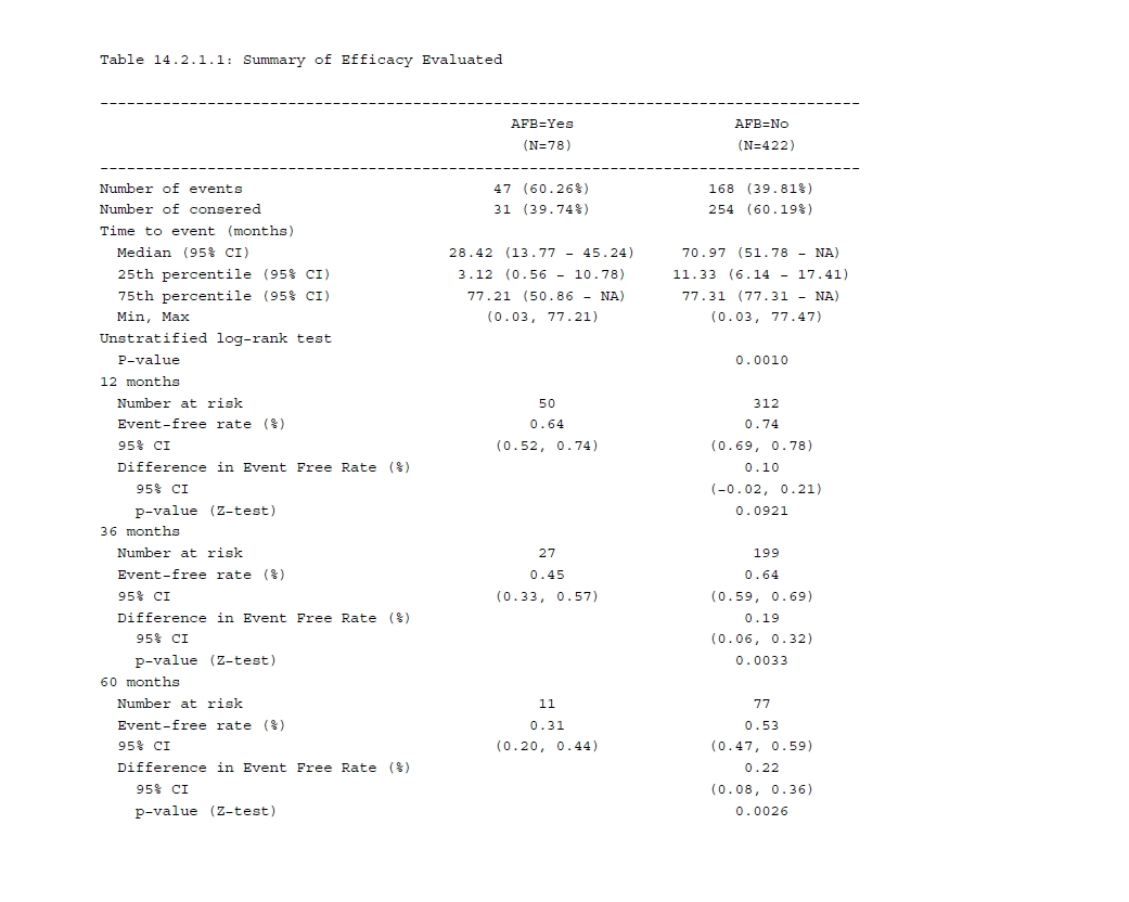
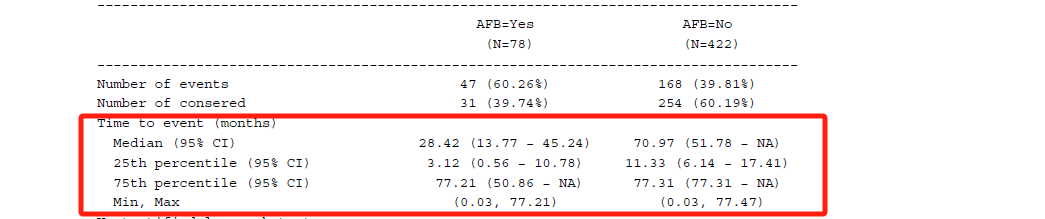
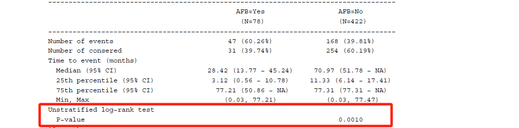
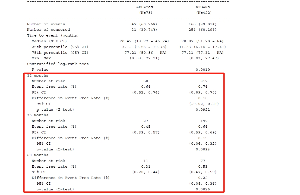
    <content type="html"><![CDATA[<p>在临床试验中，通常使用SAS来完成统计分析和生成图表，但我们不应该只局限于一种编程方法，而且这个所用的编程语言SAS并不是开源的。毫无疑问SAS能完成的事情，R和Python同样能做；但有些R和Python能做的，SAS却很难完成，我想这就是开源和不开源的区别。</p><a id="more"></a><p>之前可能只有在药厂内部的一些需求会使用R或者Python，但现在随着大药厂开始陆陆续续尝试使用R生成的结果来提交给监管机构，以及伴随着递交数据的改变（如转变成json格式），后续R或者Python在临床统计分析中应该会有一个完整的分析-呈现-递交的工作流。</p><p>以下是我对于R包<code>rtables</code>的初步尝试，比如我们想生成一张在肿瘤试验中常见的生存分析的表格，如下所示（非递交用途）。</p><figure><img src="https://www.bioinfo-scrounger.com/data/photo/rtables_tte_table.png" alt="" /><figcaption>rtables_tte_table</figcaption></figure><p>但不得不说假如真要使用<code>rtables</code>包来生成临床分析表格，最好还是搭配<code>tern</code>包来使用；前者主要是生成表格，后者则是用来分析数据，而且是无缝连接。</p><p>假如不想使用<code>tern</code>包的话，就得用另外一种使用方式，即写自定义函数来分析，然后在<code>rtables</code>的函数里调用，但这样的话就不如<code>tern</code> + <code>rtables</code>这种方式来得便捷。</p><hr /><p>步入正题，首先我先加载<code>whas500</code>数据集用于后续的生存分析（Kaplan-Meier），主要用到其中的3个变量</p><ul><li>AFB: Atrial Fibrillation (0 = No, 1 = Yes)</li><li>LENFOL: Total Length of Follow-up (Days between Date of Last Follow-up and Hospital Admission Date)</li><li>FSTAT: Vital Status at Last Follow-up (0 = Alive 1 = Dead)</li></ul><p>并对分组变量<code>AFB</code>做一些处理，拟合KM模型，其中置信区间的方法采用log-log转化</p><pre><code>library(survival)library(tidyverse)library(rtables)data(&quot;whas500&quot;, package = &quot;stabiot&quot;)dat &lt;- whas500 %&gt;%  dplyr::mutate(    AFB = case_when(      AFB == 1 ~ &quot;Yes&quot;,      TRUE ~ &quot;No&quot;    ),    AFB = factor(AFB, levels = c(&quot;Yes&quot;, &quot;No&quot;))  )km_fit &lt;- survfit(  data = dat,  formula = Surv(LENFOL, FSTAT) ~ AFB,  conf.int = 0.95,  conf.type = &quot;log-log&quot;)</code></pre><p>接着分析中位、25th和75th的生存时间以及log-rank检验，并对分析结果做一些调整使得其能更加容易匹配在<code>rtables</code>语法（即避免在<code>rtables</code>自定义函数中调整数据格式）</p><pre><code># median survival timesurv_med &lt;- summary(km_fit)$table# quantile survival timesurv_quant &lt;- quantile(km_fit, probs = c(0.25, 0.75)) %&gt;%  purrr::map(\(df) as.data.frame(df) %&gt;%    rownames_to_column(var = &quot;group&quot;)) %&gt;%  purrr::list_rbind() %&gt;%  mutate(    stat = rep(c(&quot;est&quot;, &quot;lower&quot;, &quot;upper&quot;), each = 2)  ) %&gt;%  pivot_longer(cols = c(&quot;25&quot;, &quot;75&quot;), names_to = &quot;quantile&quot;) %&gt;%  pivot_wider(    names_from = c(&quot;stat&quot;, &quot;quantile&quot;), names_glue = &quot;Q{quantile}_{stat}&quot;,    values_from = &quot;value&quot;  ) %&gt;%  column_to_rownames(var = &quot;group&quot;)# test survival curvessurv_pval &lt;- survminer::surv_pvalue(km_fit, method = &quot;log-rank&quot;)</code></pre><p>然后分析在12、36和60月时的生存率以及两组间率的比较，后者主要是通过Z检验来计算CI和P值。</p><pre><code># survival rate at 12/36/60 monthstp_cols &lt;- c(&quot;time&quot;, &quot;n.risk&quot;, &quot;n.event&quot;, &quot;n.censor&quot;, &quot;surv&quot;, &quot;std.err&quot;, &quot;lower&quot;, &quot;upper&quot;)surv_rate &lt;- summary(km_fit, times = c(12, 36, 60), extend = TRUE)[tp_cols] %&gt;%  as.data.frame() %&gt;%  split(~time) %&gt;%  purrr::map(\(df) magrittr::set_rownames(df, c(&quot;AFB=Yes&quot;, &quot;AFB=No&quot;)))# difference of survival rate by time-pointsurv_rate_diff &lt;- surv_rate %&gt;%  purrr::map(function(x){    tibble::tibble(      time = unique(x$time),      surv.diff = diff(x$surv),      std.err = sqrt(sum(x$std.err^2)),      lower = surv.diff - stats::qnorm(1 - 0.05 / 2) * std.err,      upper = surv.diff + stats::qnorm(1 - 0.05 / 2) * std.err,      pval = if (is.na(std.err)) {        NA      } else {        2 * (1 - stats::pnorm(abs(surv.diff) / std.err))      }    )  })</code></pre><p>以上是完成了分析的步骤，其实这些常规的分析步骤都已经包括在<code>tern</code>包里了。</p><hr /><p>接下来则是写自定义的函数，用于在<code>rtables</code>中的<code>analyze()</code>函数。</p><p>首先汇总两组的事件数和删失数，则需要先计算输入数据集中<code>FSTAT</code>变量的0/1分类数目，然后除以每组人数<code>.N_col</code>来得到百分比。<code>in_rows()</code>代表多行分析，即每个输入代表一行结果，<code>format</code>参数来定义输出格式</p><figure><img src="https://www.bioinfo-scrounger.com/data/photo/rtables_tte_table1.png" alt="" /><figcaption>rtables_tte_table1</figcaption></figure><pre><code>a_count_subjd &lt;- function(df, .N_col) {  in_rows(    &quot;Number of events&quot; = rcell(      sum(df$FSTAT == 1) * c(1, 1 / .N_col), format = &quot;xx (xx.xx%)&quot;     ),    &quot;Number of consered&quot; = rcell(      sum(df$FSTAT == 0) * c(1, 1 / .N_col), format = &quot;xx (xx.xx%)&quot;     )  )}</code></pre><p>接着汇总各个分位数下的生存时间估计及其CI，以及生存时间的最大最小值。在这个自定义函数中，我使用了额外参数(<code>med_tb</code>和<code>quant_tb</code>)，分别对应中位数和25th/75th分位数的数据集，其中<code>ind</code>变量可用于从上述数据集中找到对应组别的那行结果</p><figure><img src="https://www.bioinfo-scrounger.com/data/photo/rtables_tte_table2.png" alt="" /><figcaption>rtables_tte_table2</figcaption></figure><pre><code>a_surv_time_func &lt;- function(df, .var, med_tb, quant_tb) {  ind &lt;- grep(df[[.var]][1], row.names(med_tb), fixed = TRUE)  med_time = list(med_tb[ind, c(&quot;median&quot;, &quot;0.95LCL&quot;, &quot;0.95UCL&quot;)])  quantile_time = lapply(c(&quot;25&quot;, &quot;75&quot;), function(x) {    unlist(c(quant_tb[ind, grep(paste0(&quot;Q&quot;, x), names(quant_tb))]))  })  range_time = list(range(df[[&quot;LENFOL&quot;]]))  in_rows(    .list = c(med_time, quantile_time, range_time),    .names = c(      &quot;Median (95% CI)&quot;,      &quot;25th percentile (95% CI)&quot;,       &quot;75th percentile (95% CI)&quot;,      &quot;Min, Max&quot;    ),    .formats = c(      &quot;xx.xx (xx.xx - xx.xx)&quot;,      &quot;xx.xx (xx.xx - xx.xx)&quot;,      &quot;xx.xx (xx.xx - xx.xx)&quot;,      &quot;(xx.xx, xx.xx)&quot;    )  )}</code></pre><p>然后汇总两组的log-rank检验的P值，<code>pval_tb</code>对应其数据集</p><figure><img src="https://www.bioinfo-scrounger.com/data/photo/rtables_tte_table3.png" alt="" /><figcaption>rtables_tte_table3</figcaption></figure><pre><code>a_surv_pval_func &lt;- function(df, .var, .in_ref_col, pval_tb) {  in_rows(    &quot;P-value&quot; = non_ref_rcell(      pval_tb[[&quot;pval&quot;]],      .in_ref_col,      format = &quot;x.xxxx | (&lt;0.0001)&quot;    )  )}</code></pre><p>最后汇总12、36和60月时的生存率以及两组间率的比较，<code>rate_tb</code>和<code>rate_diff_tb</code>分别对应各个time point的生存率和组间率差的数据集。其中<code>non_ref_rcell()</code>可用于reference group需要为空的情况，<code>indent_mod</code>参数则可以调整缩进尺度（默认是0，即不缩进）</p><figure><img src="https://www.bioinfo-scrounger.com/data/photo/rtables_tte_table4.png" alt="" /><figcaption>rtables_tte_table4</figcaption></figure><pre><code>a_surv_rate_func &lt;- function(df, .var, .in_ref_col, rate_tb, rate_diff_tb) {  ind &lt;- grep(df[[.var]][1], row.names(rate_tb), fixed = TRUE)  in_rows(    rcell(rate_tb[ind, &quot;n.risk&quot;, drop = TRUE], format = &quot;xx&quot;),    rcell(rate_tb[ind, &quot;surv&quot;, drop = TRUE], format = &quot;xx.xx&quot;),    rcell(unlist(rate_tb[ind, c(&quot;lower&quot;, &quot;upper&quot;), drop = TRUE]), format = &quot;(xx.xx, xx.xx)&quot;),    non_ref_rcell(      rate_diff_tb[, &quot;surv.diff&quot;, drop = TRUE],      .in_ref_col,      format = &quot;xx.xx&quot;    ),    non_ref_rcell(      unlist(rate_diff_tb[, c(&quot;lower&quot;, &quot;upper&quot;), drop = TRUE]),      .in_ref_col,      format = &quot;(xx.xx, xx.xx)&quot;,      indent_mod = 1L    ),    non_ref_rcell(      rate_diff_tb[, &quot;pval&quot;, drop = TRUE],      .in_ref_col,      format = &quot;x.xxxx | (&lt;0.0001)&quot;,      indent_mod = 1L    ),    .names = c(      &quot;Number at risk&quot;,      &quot;Event-free rate (%)&quot;, &quot;95% CI&quot;,      &quot;Difference in Event Free Rate (%)&quot;, &quot;95% CI&quot;,      &quot;p-value (Z-test)&quot;    )  )}</code></pre><hr /><p>完成上述各个自定义函数后，接着是则进入<code>rtables</code>的layout部分，由于我们的这次的表格比较简单，所以所用的函数不复杂。<code>basic_table()</code>完成基本表格元素的设定，如title和footnote等；<code>split_cols_by()</code>设定表格分组变量以及定义reference group；接着就是各个分析的模块，在<code>analyze()</code>中分别调用上述的自定义函数即可，其中12/36/60月需要多次调用，因此用for循环来实现。最后用<code>build_table()</code>函数调用已完成的layout和数据集来生成最终的表格。</p><pre><code>result &lt;- basic_table(  show_colcounts = TRUE,  title = &quot;Table 14.2.1.1: Summary of Efficacy Evaluated&quot;) |&gt;  split_cols_by(&quot;AFB&quot;, ref_group = &quot;AFB=Yes&quot;) |&gt;  analyze(&quot;AFB&quot;, a_count_subjd, show_labels = &quot;hidden&quot;) |&gt;  analyze(&quot;AFB&quot;, a_surv_time_func,          var_labels = &quot;Time to event (months)&quot;, show_labels = &quot;visible&quot;,          extra_args = list(med_tb = surv_med, quant_tb = surv_quant),          table_names = &quot;kmtable&quot;  ) |&gt;  analyze(&quot;AFB&quot;, a_surv_pval_func,           var_labels = &quot;Unstratified log-rank test&quot;, show_labels = &quot;visible&quot;,          extra_args = list(pval_tb = surv_pval),          table_names = &quot;logrank&quot;  )time_point &lt;- c(12, 36, 60)for (i in seq_along(time_point)) {  result &lt;- result |&gt;    analyze(&quot;AFB&quot;, a_surv_rate_func,            var_labels = paste(time_point[i], &quot;months&quot;), show_labels = &quot;visible&quot;,            extra_args = list(rate_tb = surv_rate[[i]], rate_diff_tb = surv_rate_diff[[i]]),            table_names = paste0(&quot;timepoint_&quot;, time_point[i])    )}result |&gt;  build_table(dat %&gt;% mutate(AFB = str_c(&quot;AFB=&quot;, AFB)))</code></pre><hr /><p>以上是我对于<code>rtables</code>包的粗略理解，详细的教程可参考：<a href="https://insightsengineering.github.io/rtables/latest-tag/" target="_blank" rel="noopener">https://insightsengineering.github.io/rtables/latest-tag/</a>中的一些文档，以及一些已做分享的presentations（<a href="https://insightsengineering.github.io/rtables/latest-tag/#presentations" target="_blank" rel="noopener">https://insightsengineering.github.io/rtables/latest-tag/#presentations</a>）</p><p>现在网上关于用R语言来完成临床分析和图表生成的中文教程相对较少，希望这个简单的分享的能帮助到大家，若有出错的地方还请随时告知</p><h4 id="reference">Reference</h4><p><a href="https://insightsengineering.github.io/rtables/latest-tag/" target="_blank" rel="noopener">https://insightsengineering.github.io/rtables/latest-tag/</a><br /><a href="https://insightsengineering.github.io/tlg-catalog/stable/tables/efficacy/ttet01.html" target="_blank" rel="noopener">https://insightsengineering.github.io/tlg-catalog/stable/tables/efficacy/ttet01.html</a><br /><a href="https://pharmaverse.r-universe.dev/articles/rtables/introduction.html" target="_blank" rel="noopener">https://pharmaverse.r-universe.dev/articles/rtables/introduction.html</a><br /><a href="https://www.pharmasug.org/proceedings/japan2023/PharmaSUG-Japan-2023-05.pdf" target="_blank" rel="noopener">https://www.pharmasug.org/proceedings/japan2023/PharmaSUG-Japan-2023-05.pdf</a> <a href="https://www.r-consortium.org/all-projects/tables-in-clinical-trials-with-r#rtables" target="_blank" rel="noopener">https://www.r-consortium.org/all-projects/tables-in-clinical-trials-with-r#rtables</a></p>]]></content>
    
    <summary type="html">
    
      &lt;p&gt;在临床试验中，通常使用SAS来完成统计分析和生成图表，但我们不应该只局限于一种编程方法，而且这个所用的编程语言SAS并不是开源的。毫无疑问SAS能完成的事情，R和Python同样能做；但有些R和Python能做的，SAS却很难完成，我想这就是开源和不开源的区别。&lt;/p&gt;
    
    </summary>
    
    
      <category term="Programming-Notes" scheme="http://www.bioinfo-scrounger.com/categories/Programming-Notes/"/>
    
      <category term="R" scheme="http://www.bioinfo-scrounger.com/categories/Programming-Notes/R/"/>
    
    
      <category term="R" scheme="http://www.bioinfo-scrounger.com/tags/R/"/>
    
  </entry>
  
  <entry>
    <title>Common Survival analysis of Oncology trials in R</title>
    <link href="http://www.bioinfo-scrounger.com/archives/survival-oncology-r/"/>
    <id>http://www.bioinfo-scrounger.com/archives/survival-oncology-r/</id>
    <published>2024-03-05T14:17:34.000Z</published>
    <updated>2024-04-29T07:11:53.328Z</updated>
    
    <content type="html"><![CDATA[<p>Time-to-event endpoints are widely used in oncology trials, such as OS and PFS. And survival analysis is a common method for estimating time-to-event endpoints. In this blog, I’d like to make a note of how to summarize the essential results for survival analysis in oncology trials in R and also compare them with SAS.</p><a id="more"></a><p>Normally we will show the primary analyses, like below:</p><ul><li>Descriptive statistics of the number of events and censors.</li><li>Median (and 25th, 75th percentile) survival time from Kaplan-Meier estimate, along with 95% CI that will be calculated via Brookmeyer and Crowley methodology using log-log transformation.</li><li>Survival rate at each time-point of interest from Kaplan-Meier estimate, along with 95% CI that will be calculated via Greenwood formula using log-log transformation.</li><li>Hazard Ratio or stratified Hazard Ratio, along with 95% CI from Cox proportional hazards (PH) model, adding Efron approximation for ties handling.</li><li>P-value of log-rank test or stratified log-rank test.</li></ul><p>Above are the most prevalent survival analysis methods in the Statistical Analysis Plan (SAP) for oncology trials. Let's see how to implement them in R.</p><hr /><p>In this blog, I will use the example data from the Worcester Heart Attack Study (<a href="https://stats.idre.ucla.edu/sas/seminars/sas-survival/" target="_blank" rel="noopener">https://stats.idre.ucla.edu/sas/seminars/sas-survival/</a>) with 500 subjects, which has been wrapped in <code>stabiot</code> R package. And you can find the description of all columns in <code>?whas500</code> after installing the package, like <code>devtools::install_github("kaigu1990/stabiot")</code>.</p><pre><code>library(survival)library(stabiot)data(&quot;whas500&quot;)</code></pre><p>If we want to compare the survival time between the subjects with and without atrial fibrillation, we should first convert the <code>AFB</code> variable to a factor.</p><pre><code>dat &lt;- whas500 %&gt;%  mutate(    AFB = factor(AFB, levels = c(1, 0))  )</code></pre><h4 id="kaplan-meier-estimate">Kaplan-Meier estimate</h4><p>Afterwards we can compute the Kaplan-Meier estimate of the survival function for the <code>whas500</code> dataset.</p><pre><code>fit_km &lt;- survfit(Surv(LENFOL, FSTAT) ~ AFB, data = dat, conf.type = &quot;log-log&quot;)</code></pre><p>In the <code>Surv()</code> function, the event variable takes on the value 1 for events and 0 for censoring, which is in contrast to SAS. And the <code>conf.type = "log-log"</code> tells the function to estimate the CI of median or other percentiles via Brookmeyer and Crowley methodology using log-log transformation because the default argument is <code>conf.type = "log"</code>.</p><p>Then we can use <code>summary()</code> to see more detail or obtain the median survival time.</p><pre><code>print(summary(fit_km), digits = 4)# median survival time with CIsummary(fit_km)$table##       records n.max n.start events    rmean se(rmean)   median  0.95LCL  0.95UCL## AFB=1      78    78      78     47 35.86989  3.821604 28.41889 13.76591 45.24025## AFB=0     422   422     422    168 48.63073  1.714196 70.96509 51.77823       NA</code></pre><p>Or use <code>quantile()</code> for any quantile estimate.</p><pre><code># 25% 50% and 75% survival time and CIquantile(fit_km, probs = c(0.25, 0.5, 0.75)) ## $quantile##             25       50       75## AFB=1  3.12115 28.41889 77.20739## AFB=0 11.33470 70.96509 77.30595## ## $lower##              25       50       75## AFB=1 0.5585216 13.76591 50.85832## AFB=0 6.1437372 51.77823 77.30595## $upper##             25       50 75## AFB=1 10.77618 45.24025 NA## AFB=0 17.41273       NA NA</code></pre><p>If you want to know the survival rate at specific time points like 12, 24 and 36 months, use <code>times = c(12, 36, 60)</code> in the <code>summary()</code> function.</p><pre><code>summary(fit_km, times = c(12, 36, 60))## Call: survfit(formula = Surv(LENFOL, FSTAT) ~ AFB, data = dat, conf.type = &quot;log-log&quot;)## ##                 AFB=1 ##  time n.risk n.event survival std.err lower 95% CI upper 95% CI##    12     50      28    0.641  0.0543        0.524        0.736##    36     27      12    0.455  0.0599        0.335        0.567##    60     11       6    0.315  0.0643        0.195        0.441## ##                 AFB=0 ##  time n.risk n.event survival std.err lower 95% CI upper 95% CI##    12    312     110    0.739  0.0214        0.695        0.779##    36    199      32    0.645  0.0244        0.595        0.690##    60     77      21    0.530  0.0311        0.467        0.589</code></pre><p>The <code>n.risk</code> column gives us the number of subjects who are still in the risk condition at specific time points. The <code>n.event</code> column demonstrates the number of events that occurred at the time. And <code>survival</code> column tells us the survival rate from the KM estimate and the last two columns are the corresponding CI.</p><p>In addition, you may be interested in the difference rate and corresponding CI between groups with and without AFB. Now that you know the rate and SE for two groups seperately, thus the difference rate and difference SE can be simply calculated. Afterwards for CI calculation, utilize the <code>qnorm()</code> function as follows.</p><pre><code>diff_rate &lt;- diff(rate_tb$surv)diff_se &lt;- sqrt(sum(rate_tb$std.err^2))diff_rate + c(-1, 1) * qnorm(1 - 0.05 / 2) * diff_se## [1] -0.01608841  0.21271012</code></pre><h4 id="log-rank-test">Log-rank test</h4><p>The Log-rank test is a non-parametric test for comparing the survival function across two or more groups where the null hypothesis is that the groups's survival functions are the same. It can be calculated via <code>survminer::surv_pvalue()</code> function with <code>method = "log-rank"</code> for <code>survfit</code> object, or <code>survival::survdiff()</code> function with <code>rho = 0</code>. Both are part of the default set, so you don't need to define them explicitly. Let me show them separately, as shown below.</p><pre><code>survminer::surv_pvalue(fit_km, method = &quot;log-rank&quot;)##   variable         pval   method    pval.txt## 1      AFB 0.0009616214 Log-rank p = 0.00096survival::survdiff(Surv(LENFOL, FSTAT) ~ AFB, data = dat, rho = 0)$pvalue## [1] 0.0009616214</code></pre><p>If you would like to know what is the Log rank test, this article (<a href="https://datatab.net/tutorial/log-rank-test" target="_blank" rel="noopener">Log Rank Test</a>) can be for your reference.</p><h4 id="cox-ph-model">Cox PH model</h4><p>As we will know, the Cox regression model is a semi-parametric model since it makes no assumption about the distribution of the event times that is similar to the KM method of non-parametric, but it relies on a partial likelihood estimation that is partially defined parametrically. Before fitting the Cox model, we should make sure the proportional hazard assumption is met. And more details can be seen at <a href="http://www.sthda.com/english/wiki/cox-model-assumptions" target="_blank" rel="noopener">http://www.sthda.com/english/wiki/cox-model-assumptions</a>.</p><p>Let's go on the <code>whas500</code> example data. If you want to estimate the hazard ratio comparing those two groups and also specify the efron approximation for tie handling, the <code>survival::coxph()</code> function can be used for fitting Cox PH models simply.</p><pre><code>fit_cox &lt;- coxph(Surv(LENFOL, FSTAT) ~ AFB, data = dat, ties = &quot;efron&quot;)## Call:## coxph(formula = Surv(LENFOL, FSTAT) ~ AFB, data = dat, ties = &quot;efron&quot;)## ##   n= 500, number of events= 215 ## ##         coef exp(coef) se(coef)      z Pr(&gt;|z|)   ## AFB0 -0.5397    0.5829   0.1654 -3.263   0.0011 **## ---## Signif. codes:  0 ‘***’ 0.001 ‘**’ 0.01 ‘*’ 0.05 ‘.’ 0.1 ‘ ’ 1## ##      exp(coef) exp(-coef) lower .95 upper .95## AFB0    0.5829      1.716    0.4215    0.8061## ## Concordance= 0.537  (se = 0.014 )## Likelihood ratio test= 9.58  on 1 df,   p=0.002## Wald test            = 10.64  on 1 df,   p=0.001## Score (logrank) test = 10.9  on 1 df,   p=0.001</code></pre><p>The Cox results can be interpreted as follows: - The <code>coef</code> is the coefficient, and <code>z</code> is the Wald statistic value that corresponds to the rate of <code>coef</code> to its standard error (<code>se(coef)</code>). - Hazard ratio (HR) corresponds to the <code>exp(coef)</code>, which is comparing the current level to the reference level. So the HR of <code>0.58</code> indicates that the subjects without AFB have 0.58 less hazard or risk compared to those who have AFB. In other words, if the event occurred in 20% of the no AFB group, it would occur in 8.4% (20% - (20% x 0.58)) of the AFB group, which means the no AFB can reduce the hazard of deaths by 0.58. - The HR confidence interval is also provided, with lower 95% bound of 0.4215 and upper 95% bound of 0.8061. - There are three alternative tests for overall significance of the model: likelihood-ratio test, Wald test, and score log-rank statistics. And as we know, log-rank test is a special case of Cox model, which means it equals a univariate Cox regression (only considering treatment). So we can calculate the log-rank p-value from 'survdiff()` as well for the Cox model.</p><h4 id="stratified-log-rank-test-and-cox-ph-model">Stratified Log-rank test and Cox PH model</h4><p>The stratified log-rank test is commonly used for randomized clinical trials when there are baseline factors that may be related to the treatment effect.</p><blockquote><p>The stratified log-rank test is the log-rank test that accounts for the difference in prognostic factors between the two groups. Specifically, we divide the data according to the levels of the significant prognostic factors and form a stratum for each level. At each level, we arrange the survival times in ascending order and calculate the observed number of events, expected number of events, and variance at each survival time as we would in the regular log-rank test. (<a href="https://www.sciencedirect.com/science/article/abs/pii/B9780123821676000230" target="_blank" rel="noopener">Chapter 23 - An Introduction to Survival Analysis</a>)</p></blockquote><p>To implement the stratified log-rank test, simply include the <code>strata()</code> within the survival model formula as follows.</p><pre><code>strat_km &lt;- survfit(Surv(LENFOL, FSTAT) ~ AFB + strata(AGE, GENDER), data = dat, conf.type = &quot;log-log&quot;)survminer::surv_pvalue(strat_km, method = &quot;log-rank&quot;)##                  variable       pval   method  pval.txt## 1 AFB+strata(AGE, GENDER) 0.08269744 Log-rank p = 0.083</code></pre><p>Regarding the stratified Cox model, it can be used if there are one or more predictors that don’t satisfy the proportional hazard assumptions. In other words, the proportional hazard is violated.</p><p>It can also be performed using <code>coxph</code> along with <code>strata()</code> function, the same as stratified log-rank test.</p><pre><code>strat_cox &lt;- coxph(Surv(LENFOL, FSTAT) ~ AFB + strata(AGE, GENDER), data = dat, ties = &quot;efron&quot;)summary(strat_cox)strat_cox %&gt;%   broom::tidy(exponentiate = TRUE, conf.int = TRUE, conf.level = 0.95) %&gt;%  select(term, estimate, conf.low, conf.high)## # A tibble: 1 × 4##   term  estimate conf.low conf.high##   &lt;chr&gt;    &lt;dbl&gt;    &lt;dbl&gt;     &lt;dbl&gt;## 1 AFB0     0.695    0.462      1.05</code></pre><p>Above is a summary of common survival analyses in R. In the next step, I would like to wrap these functions into one or two functions and specify the print method so that we can simply use them to compare with SAS.</p><h4 id="reference">Reference</h4><p><a href="https://stats.stackexchange.com/questions/486806/the-logrank-test-statistic-is-equivalent-to-the-score-of-a-cox-regression-is-th" target="_blank" rel="noopener">https://stats.stackexchange.com/questions/486806/the-logrank-test-statistic-is-equivalent-to-the-score-of-a-cox-regression-is-th</a><br /><a href="https://discourse.datamethods.org/t/when-is-log-rank-preferred-over-univariable-cox-regression/2344" target="_blank" rel="noopener">https://discourse.datamethods.org/t/when-is-log-rank-preferred-over-univariable-cox-regression/2344</a><br /><a href="https://www.bookdown.org/rwnahhas/RMPH/survival-cox-fit.html" target="_blank" rel="noopener">Introduction to Regression Methods for Public Health Using R</a><br /><a href="https://www.drizopoulos.com/courses/emc/basic_surivival_analysis_in_r" target="_blank" rel="noopener">Survival Analysis in R Companion</a><br /><a href="https://psiaims.github.io/CAMIS/R/survival.html" target="_blank" rel="noopener">Survival Analysis Using R</a><br /><a href="https://towardsdatascience.com/survival-analysis-in-clinical-trials-log-rank-test-8f1229e7f0f0" target="_blank" rel="noopener">Survival analysis in clinical trials — Log-rank test</a><br /><a href="https://towardsdatascience.com/survival-analysis-in-clinical-trials-f87b8cbc2b1a" target="_blank" rel="noopener">Survival analysis in clinical trials — Kaplan-Meier estimator</a></p>]]></content>
    
    <summary type="html">
    
      &lt;p&gt;Time-to-event endpoints are widely used in oncology trials, such as OS and PFS. And survival analysis is a common method for estimating time-to-event endpoints. In this blog, I’d like to make a note of how to summarize the essential results for survival analysis in oncology trials in R and also compare them with SAS.&lt;/p&gt;
    
    </summary>
    
    
      <category term="Biometrics" scheme="http://www.bioinfo-scrounger.com/categories/Biometrics/"/>
    
      <category term="BiomedicalStats" scheme="http://www.bioinfo-scrounger.com/categories/Biometrics/BiomedicalStats/"/>
    
    
      <category term="Statistics" scheme="http://www.bioinfo-scrounger.com/tags/Statistics/"/>
    
  </entry>
  
  <entry>
    <title>Evaluation of Best Overall Response per RECIST in R</title>
    <link href="http://www.bioinfo-scrounger.com/archives/bor_recist/"/>
    <id>http://www.bioinfo-scrounger.com/archives/bor_recist/</id>
    <published>2024-02-28T16:51:20.000Z</published>
    <updated>2024-02-28T16:54:09.678Z</updated>
    
    <content type="html"><![CDATA[<p>The Best Overall Response (BOR) is a very common evaluation of efficacy in oncology trials. Usually, it is defined as the best response among all time-point responses from the treatment start until the first disease progression, in the order of CR, PR, SD, PD, and NE per RECIST 1.1. For non-randomized trials, BOR is not only the best among all responses but also requires confirmation for CR and PR to ensure the result is not a measurement error. More details can be found in the RECIST 1.1 document, which I will not expand on here.</p><a id="more"></a><p>Although there are lots of blogs on Google that will tell you how to derive BOR in SAS, only a few people will use R to do so. This article is to talk about how to implement BOR with or without confirmation in R.</p><h4 id="best-overall-response-without-confirmation">Best Overall Response without confirmation</h4><p>Firstly, let's look at the programming logic for BOR without confirmation.</p><ul><li>Set to complete response (CR) if one CR exists.</li><li>Set to partial response (PR) if one PR exists .</li><li>Set to stable disease (SD) if one SD exists, which meets the minimum requirement for SD duration from treatment (or randomization) start to the date of the response.</li><li>Set to progressive disease (PD) if one PD exists.</li><li>Set to not estimable (NE) if only NE exists or the response cannot meet minimum SD duration criteria.</li></ul><p>Afterwards, you can select the best response above for each subject as the BOR.</p><h4 id="best-overall-response-with-confirmation">Best Overall Response with confirmation</h4><p>Below are the rules to evaluate the best response where the confirmation of CR and PR is required for BOR deviation, from RECIST guideline (<a href="https://ctep.cancer.gov/protocolDevelopment/docs/recist_guideline.pdf" target="_blank" rel="noopener">https://ctep.cancer.gov/protocolDevelopment/docs/recist_guideline.pdf</a>)</p><figure><img src="https://www.bioinfo-scrounger.com/data/photo/confirmed_BOR.png" alt="" /><figcaption>confirmed_BOR</figcaption></figure><p>Actually, we don't consider the scenario where the CR is followed by PR, but we must consider the scenario where subsequent response is not sequential. And we also need to consider how many NEs are acceptable between response and confirmatory response.</p><p>Thus the programming logic for confirmed BOR can be summarized as following:</p><ul><li>Set to complete response (CR) if there is one confirmatory CR at least a minimum number of days (e.g., 28 days) later, all responses between the two should only be "CR" or "NE", and there are no more than a maximum NE (e.g., one NE) between two responses.</li><li>Set to partial response (PR) if there is one confirmatory CR or PR at least a minimum number of days (e.g., 28 days) later, all responses between the two should only be are "CR", "PR" or "NE", and there are no more than a maximum NE (e.g., one NE) between two PR/CR responses.</li><li>Set to stable disease (SD) if there is one CR, PR or SD that meets the minimum requirement for the duration from treatment (or randomization) start to the date of that response.</li><li>Set to progressive disease (PD) if one PD exists.</li><li>Set to not estimable (NE) if there is at least one CR, PR, SD, NE.</li></ul><p>And then like the unconfirmed BOR, you can select the best response above for each subject as the confirmed BOR.</p><h4 id="how-to-implement-it-in-r">How to implement it in R</h4><p>I have created a function in <code>stabiot</code> R package following the rules we discussed above. For example, let's try it using the <code>derive_bor()</code> function as shown below. More detials can be found in <code>?derive_bor</code>.</p><pre><code># This example is referred from `admiral::event_joined`.adrs &lt;- tibble::tribble(  ~USUBJID, ~TRTSDTC,     ~ADTC,        ~AVALC,  &quot;1&quot;,      &quot;2020-01-01&quot;, &quot;2020-01-01&quot;, &quot;PR&quot;,  &quot;1&quot;,      &quot;2020-01-01&quot;, &quot;2020-02-01&quot;, &quot;CR&quot;,  &quot;1&quot;,      &quot;2020-01-01&quot;, &quot;2020-02-16&quot;, &quot;NE&quot;,  &quot;1&quot;,      &quot;2020-01-01&quot;, &quot;2020-03-01&quot;, &quot;CR&quot;,  &quot;1&quot;,      &quot;2020-01-01&quot;, &quot;2020-04-01&quot;, &quot;SD&quot;,  &quot;2&quot;,      &quot;2019-12-12&quot;, &quot;2020-01-01&quot;, &quot;SD&quot;,  &quot;2&quot;,      &quot;2019-12-12&quot;, &quot;2020-02-01&quot;, &quot;PR&quot;,  &quot;2&quot;,      &quot;2019-12-12&quot;, &quot;2020-03-01&quot;, &quot;SD&quot;,  &quot;2&quot;,      &quot;2019-12-12&quot;, &quot;2020-03-13&quot;, &quot;CR&quot;,  &quot;4&quot;,      &quot;2019-12-30&quot;, &quot;2020-01-01&quot;, &quot;PR&quot;,  &quot;4&quot;,      &quot;2019-12-30&quot;, &quot;2020-03-01&quot;, &quot;NE&quot;,  &quot;4&quot;,      &quot;2019-12-30&quot;, &quot;2020-04-01&quot;, &quot;NE&quot;,  &quot;4&quot;,      &quot;2019-12-30&quot;, &quot;2020-05-01&quot;, &quot;PR&quot;,  &quot;5&quot;,      &quot;2020-01-01&quot;, &quot;2020-01-01&quot;, &quot;PR&quot;,  &quot;5&quot;,      &quot;2020-01-01&quot;, &quot;2020-01-10&quot;, &quot;PR&quot;,  &quot;5&quot;,      &quot;2020-01-01&quot;, &quot;2020-01-20&quot;, &quot;PR&quot;,  &quot;6&quot;,      &quot;2020-02-02&quot;, &quot;2020-02-06&quot;, &quot;PR&quot;,  &quot;6&quot;,      &quot;2020-02-02&quot;, &quot;2020-02-16&quot;, &quot;CR&quot;,  &quot;6&quot;,      &quot;2020-02-02&quot;, &quot;2020-03-30&quot;, &quot;PR&quot;,  &quot;7&quot;,      &quot;2020-02-02&quot;, &quot;2020-02-06&quot;, &quot;PR&quot;,  &quot;7&quot;,      &quot;2020-02-02&quot;, &quot;2020-02-16&quot;, &quot;CR&quot;,  &quot;7&quot;,      &quot;2020-02-02&quot;, &quot;2020-04-01&quot;, &quot;NE&quot;,  &quot;8&quot;,      &quot;2020-02-01&quot;, &quot;2020-02-16&quot;, &quot;PD&quot;) %&gt;%  dplyr::mutate(    ADT = lubridate::ymd(ADTC),    TRTSDT = lubridate::ymd(TRTSDTC),    PARAMCD = &quot;OVR&quot;,    PARAM = &quot;Overall Response by Investigator&quot;  ) %&gt;%  dplyr::select(-TRTSDTC)</code></pre><p>Suppose that we want to calculate the BOR without confirmation and the SD duration is set to 4 weeks, only we simply need to specify <code>ref_start_window = 28</code>.</p><pre><code>derive_bor(data = adrs, ref_start_window = 28)## # A tibble: 7 × 8##   USUBJID ADTC       AVALC ADT        TRTSDT     PARAMCD PARAM                  AVAL##   &lt;chr&gt;   &lt;chr&gt;      &lt;chr&gt; &lt;date&gt;     &lt;date&gt;     &lt;chr&gt;   &lt;chr&gt;                 &lt;dbl&gt;## 1 1       2020-02-01 CR    2020-02-01 2020-01-01 BOR     Best Overall Response     1## 2 2       2020-03-13 CR    2020-03-13 2019-12-12 BOR     Best Overall Response     1## 3 4       2020-01-01 PR    2020-01-01 2019-12-30 BOR     Best Overall Response     2## 4 5       2020-01-01 PR    2020-01-01 2020-01-01 BOR     Best Overall Response     2## 5 6       2020-02-16 CR    2020-02-16 2020-02-02 BOR     Best Overall Response     1## 6 7       2020-02-16 CR    2020-02-16 2020-02-02 BOR     Best Overall Response     1## 7 8       2020-02-16 PD    2020-02-16 2020-02-01 BOR     Best Overall Response     4</code></pre><p>Suppose that we want to calculate the BOR with confirmation and the SD duration is set to 4 weeks, and the interval of two responses is set to 28 days, we simply need to add <code>ref_interval = 28</code> and <code>confirm = TRUE</code></p><pre><code>derive_bor(data = adrs, ref_start_window = 28, ref_interval = 28, confirm = TRUE)## # A tibble: 7 × 8##   USUBJID ADTC       AVALC ADT        TRTSDT     PARAMCD PARAM                            AVAL##   &lt;chr&gt;   &lt;chr&gt;      &lt;chr&gt; &lt;date&gt;     &lt;date&gt;     &lt;chr&gt;   &lt;chr&gt;                           &lt;dbl&gt;## 1 1       2020-02-01 CR    2020-02-01 2020-01-01 CBOR    Confirmed Best Overall Response     1## 2 2       2020-02-01 SD    2020-02-01 2019-12-12 CBOR    Confirmed Best Overall Response     3## 3 4       2020-05-01 SD    2020-05-01 2019-12-30 CBOR    Confirmed Best Overall Response     3## 4 5       2020-01-01 NE    2020-01-01 2020-01-01 CBOR    Confirmed Best Overall Response     5## 5 6       2020-02-06 PR    2020-02-06 2020-02-02 CBOR    Confirmed Best Overall Response     2## 6 7       2020-02-06 NE    2020-02-06 2020-02-02 CBOR    Confirmed Best Overall Response     5## 7 8       2020-02-16 PD    2020-02-16 2020-02-01 CBOR    Confirmed Best Overall Response     4</code></pre><p>If we don't want any NE between the response and confirmatory response in addition to the above conditions, we can simply add <code>max_ne = 0</code>.</p><pre><code>derive_bor(data = adrs, ref_start_window = 28, ref_interval = 28, confirm = TRUE, max_ne = 0)## # A tibble: 7 × 8##   USUBJID ADTC       AVALC ADT        TRTSDT     PARAMCD PARAM                            AVAL##   &lt;chr&gt;   &lt;chr&gt;      &lt;chr&gt; &lt;date&gt;     &lt;date&gt;     &lt;chr&gt;   &lt;chr&gt;                           &lt;dbl&gt;## 1 1       2020-01-01 PR    2020-01-01 2020-01-01 CBOR    Confirmed Best Overall Response     2## 2 2       2020-02-01 SD    2020-02-01 2019-12-12 CBOR    Confirmed Best Overall Response     3## 3 4       2020-05-01 SD    2020-05-01 2019-12-30 CBOR    Confirmed Best Overall Response     3## 4 5       2020-01-01 NE    2020-01-01 2020-01-01 CBOR    Confirmed Best Overall Response     5## 5 6       2020-02-06 PR    2020-02-06 2020-02-02 CBOR    Confirmed Best Overall Response     2## 6 7       2020-02-06 NE    2020-02-06 2020-02-02 CBOR    Confirmed Best Overall Response     5## 7 8       2020-02-16 PD    2020-02-16 2020-02-01 CBOR    Confirmed Best Overall Response     4</code></pre><p>The above all are my summries for BOR calculation. If there is any problem or error, please email me to let me know, or leave your issues in the <a href="https://github.com/kaigu1990/stabiot/issues" target="_blank" rel="noopener">https://github.com/kaigu1990/stabiot/issues</a>.</p><p>At the very least, I'd like to appreciate the <code>admiral</code> R package, I have learned more programming skills for BOR calculation from <code>admiral::derive_extreme_event()</code>.</p><h4 id="reference">Reference</h4><p>https://github.com/pharmaverse/admiral<br />https://www.pharmasug.org/proceedings/2023/QT/PharmaSUG-2023-QT-047.pdf<br />https://www.pharmasug.org/proceedings/2020/DV/PharmaSUG-2020-DV-066.pdf<br />https://ctep.cancer.gov/protocolDevelopment/docs/recist_guideline.pdf<br />https://www.lexjansen.com/pharmasug-cn/2021/SR/Pharmasug-China-2021-SR038.pdf</p>]]></content>
    
    <summary type="html">
    
      &lt;p&gt;The Best Overall Response (BOR) is a very common evaluation of efficacy in oncology trials. Usually, it is defined as the best response among all time-point responses from the treatment start until the first disease progression, in the order of CR, PR, SD, PD, and NE per RECIST 1.1. For non-randomized trials, BOR is not only the best among all responses but also requires confirmation for CR and PR to ensure the result is not a measurement error. More details can be found in the RECIST 1.1 document, which I will not expand on here.&lt;/p&gt;
    
    </summary>
    
    
      <category term="Biometrics" scheme="http://www.bioinfo-scrounger.com/categories/Biometrics/"/>
    
      <category term="BiomedicalStats" scheme="http://www.bioinfo-scrounger.com/categories/Biometrics/BiomedicalStats/"/>
    
    
      <category term="Statistics" scheme="http://www.bioinfo-scrounger.com/tags/Statistics/"/>
    
  </entry>
  
  <entry>
    <title>Response Rate and Odd Ratio in R and SAS</title>
    <link href="http://www.bioinfo-scrounger.com/archives/orr_odds_ratio/"/>
    <id>http://www.bioinfo-scrounger.com/archives/orr_odds_ratio/</id>
    <published>2024-01-22T14:40:49.000Z</published>
    <updated>2024-04-22T08:33:28.180Z</updated>
    
    <content type="html"><![CDATA[<p>As we know, the objective response rate (ORR) is used as a key endpoint to demonstrate the efficacy of a treatment in oncology and is also valuable for clinical decision making in phase I-II trials, especially in single-arm trials.</p><a id="more"></a><p>The advantage of the ORR is that it can be assessed earlier than PFS/OS, and in smaller samples. In general, we will assume that the response rate follows the binomial distribution, so naturally we will consider the ORR as a binomial response rate, and the Clopper-Pearson method is frequently used to estimate the two-sided 95% confidence interval (CI). If you would like to control the confounding factors in the stratified study design, the Cochran-Mantel-Haenszel (CMH) test provides a solution to address these needs.</p><p>How about the odds ratio (OR)? It is a measure of the association between an exposure and an outcome. So it can be regarded as the odds of the outcome occurring in a particular exposure compared to the odds in the absence of that exposure. Thus, we can use it to assess the ORR between the treatment and control groups in RCT trials in combination with a 95% binomial response rate as presented in reports. More details can be found in <a href="https://www.ncbi.nlm.nih.gov/pmc/articles/PMC2938757/" target="_blank" rel="noopener">Explaining Odds Ratios</a>.</p><h4 id="orr-and-or-in-sas">ORR and OR in SAS</h4><p>Firstly, let's see how to use <code>proc freq</code> in SAS to obtain the ORR rate with Clopper-Pearson (Exact) CI and the odds ratio with and without stratification. Imaging we have an example of data with columns like TRTPN(1/2), ORR(1 for subjects with ORR and 0 without ORR), Strata1(A/B) and the count number.</p><pre><code>data dat;    input TRTPN ORR Strata1 $ Count @@;    datalines;1 1 A 8  1 1 B 121 2 A 17 1 2 B 132 1 A 13 2 1 B 92 2 A 20 2 2 B 8;run;</code></pre><p>Then use the <code>tables</code> statement with <code>binomial</code> to compute the CI of ORR. The <code>level="1"</code> binomial option can help you compute the proportion for subjects with events, which means the CI corresponds to the ORR event. And the <code>exact biomial</code> can compute the Clopper-Pearson CI as you need.</p><pre><code>ods listing close;proc freq data=dat;    by trtpn;    weight count/zeros;    tables orr/binomial(level=&quot;1&quot;) alpha=0.05;    exact binomial;    ods output binomial=orrci;run;ods listing;</code></pre><p>Before the stratification analysis, let's see the common odds ratio without any stratified factors. The option <code>chisq</code> requests chi-square tests and measurements, and <code>relrisk</code> displays the odds ratio and relative risk with asymptotic Wald CI by default.</p><pre><code>ods listing close;proc freq data=dat;    weight count/zeros;    tables TRTPN*ORR /chisq relrisk;    ods output FishersExact=pval RelativeRisks=ci;run;ods listing;</code></pre><p>And then let's see how to use <code>CMH</code> as the statistical method in <code>proc freq</code> to obtain the association statistics, p-value of Cochran-Mantel-Haenszel test, adjusted odds ratio by Strata1 variable and corresponding CI.</p><pre><code>ods listing close;proc freq data=dat;    weight count/zeros;    tables Strata1*TRTPN*ORR /cmh;    ods output cmh=cmhpval CommonRelRisks=cmhci; run;</code></pre><p>Now that we have seen the example of the <code>proc freq</code> used to compute the odds ratio with and without stratification, let's have a look at how to use the logistic regression <code>proc logistic</code> to do it.</p><pre><code>proc logistic data=dat;    weight count;    class TRTPN / param=ref ref=last;    model ORR(event=&#39;1&#39;)=TRTPN;run;</code></pre><p>And the stratification analysis by logistic as shown below.</p><pre><code>proc logistic data=dat;    freq count;    class TRTPN Strata1 / param=ref ref=last;    strata Strata1;    model ORR(event=&#39;1&#39;)=TRTPN;run;</code></pre><p>However, we can see there is a little difference between <code>proc freq</code> and the logistic regression method of odds ratio. The same condition occurs in R as well.</p><h4 id="orr-and-or-in-r">ORR and OR in R</h4><p>Now let's jump into the R section, how can we handle the same analysis in R?</p><p>First of all, I want to recommend the <code>tern</code> R package, which focuses on clinical statistical analysis and provides serveral helpful functions. More details can be found in the <a href="https://insightsengineering.github.io/tern/latest-tag/" target="_blank" rel="noopener">tern package document</a>.</p><p>I create an example data set similar to the one shown above, which includes the same columns but is not the counted table. The columns of strata1 - strata3 represent three stratified factors.</p><pre><code>set.seed(12)dta &lt;- data.frame(  orr = sample(c(1, 0), 100, TRUE),  trtpn = factor(rep(c(1, 2), each = 50), levels = c(2, 1)),  strata1 = factor(sample(c(&quot;A&quot;, &quot;B&quot;), 100, TRUE)),  strata2 = factor(sample(c(&quot;C&quot;, &quot;D&quot;), 100, TRUE)),  strata3 = factor(sample(c(&quot;E&quot;, &quot;F&quot;), 100, TRUE)))</code></pre><p>Then you can use <code>BinomCI</code> function to compute the CI of ORR and <code>BinomDiffCI</code> function to compute the CI of difference ORR in two treatments.</p><pre><code>dta %&gt;% count(trtpn, orr)##   trtpn orr  n## 1     2   0 28## 2     2   1 22## 3     1   0 30## 4     1   1 20    DescTools::BinomCI(x = 20, n = 50, method = &quot;clopper-pearson&quot;)##      est    lwr.ci   upr.ci## [1,] 0.4 0.2640784 0.548206DescTools::BinomDiffCI(20, 50, 22, 50, method=c(&quot;wald&quot;))##        est     lwr.ci    upr.ci## [1,] -0.04 -0.2333125 0.1533125</code></pre><p>Regarding the unstratification analysis of odds ratio, we can use <code>DescTools::OddsRatio()</code> function, or logistic regression using <code>glm()</code> with <code>logit</code> link. Below is the code to get the odds ratio and corresponding Wald CI using <code>OddsRatio()</code> function.</p><pre><code>DescTools::OddsRatio(matrix(c(20, 22, 30, 28), nrow = 2, byrow = TRUE),  method = &quot;wald&quot;, conf.level = 0.95)## odds ratio     lwr.ci     upr.ci ##  0.8484848  0.3831831  1.8788054 </code></pre><p>And the <code>glm()</code> function also can get the same results as shwon below.</p><pre><code>fit &lt;- glm(orr ~ trtpn, data = dta, family = binomial(link = &quot;logit&quot;))exp(cbind(Odds_Ratio = coef(fit), confint(fit)))##             Odds_Ratio     2.5 %   97.5 %## (Intercept)  0.7857143 0.4450719 1.369724## trtpn1       0.8484848 0.3811997 1.879735</code></pre><p>Regarding the unstratification analysis of odds ratio, there are two ways that I have found for computing it. One is Cochran-Mantel-Haenszel chi-squared test using <code>mantelhaen.test()</code> function, and another is conditional logistic regression <code>survival::clogit()</code> function with <code>strata</code> usage for stratification analysis. Let's have a look at the specific steps.</p><p>Assuming that we want to consider three stratified factors in our CMH test, we'd better to pre-process data properly before we pass on to <code>mantelhaen.test</code> function. Because this function has certain requirement for the input data format.</p><pre><code># pre-processdf &lt;- dta %&gt;% count(trtpn, orr, strata1, strata2, strata3)tab &lt;- xtabs(n ~ trtpn + orr + strata1 + strata2 + strata3, data = df)tb &lt;- as.table(array(c(tab), dim = c(2, 2, 2 * 2 * 2)))# CMH analysismantelhaen.test(tb, correct = FALSE)## Mantel-Haenszel chi-squared test without continuity correction## data:  tb## Mantel-Haenszel X-squared = 0.40574, df = 1, p-value = 0.5241## alternative hypothesis: true common odds ratio is not equal to 1## 95 percent confidence interval:##  0.3376522 1.7320849## sample estimates:## common odds ratio ##         0.7647498</code></pre><p>PS. If we only use one stratification like <code>strata1</code>, the same result as SAS <code>proc freq</code> we can get here. Besides you can also use <code>vcdExtra::CMHtest</code> to compute the p-value of CMH, but if you want to obtain the same p-value used in SAS, a modification has to be made to the vcdExtra library. Refer to this github issue: <a href="https://github.com/friendly/vcdExtra/issues/3" target="_blank" rel="noopener">https://github.com/friendly/vcdExtra/issues/3</a>.</p><p>And then how to implement it using conditional logistic regression, just add the <code>strata</code> in the formula.</p><pre><code>library(survival)fit &lt;- clogit(formula = orr ~ trtpn + strata(strata1, strata2, strata3), data = dta)exp(cbind(Odds_Ratio = coef(fit), confint(fit)))##        Odds_Ratio    2.5 %   97.5 %## trtpn1  0.7592608 0.335024 1.720704</code></pre><h4 id="summary">Summary</h4><p>Above all, here is my brief summary for the statisical analysis of ORR and odds ratio in R and SAS. And CMH is also a widely used method to test the association between treatment and binary outcome when you want to consider the stratification factors. Lastly, a question remain unanswered: why do we obtain different results from the logistic regression compared to the CMH test when we apply them to compute the the stratified odds ratio. I'm looking for how to respond to it.</p><h4 id="reference">Reference</h4><p><a href="https://insightsengineering.github.io/tern/latest-tag/articles/tern.html" target="_blank" rel="noopener">Introduction to tern</a> <a href="https://www.pharmasug.org/proceedings/2020/SA/PharmaSUG-2020-SA-051.pdf" target="_blank" rel="noopener">Calculation of Cochran–Mantel–Haenszel Statistics for Objective Response and Clinical Benefit Rates and the Effects of Stratification Factors</a><br /><a href="https://www.lexjansen.com/pharmasug-cn/2021/CC/Pharmasug-China-2021-CC076.pdf" target="_blank" rel="noopener">Estimating Binomial Proportion Confidence Interval with Zero Frequency Response using FREQ Procedure</a><br /><a href="https://www.pharmasug.org/proceedings/2014/SP/PharmaSUG-2014-SP13.pdf" target="_blank" rel="noopener">The path less trodden - PROC FREQ for ODDS RATIO</a><br /><a href="https://www.statology.org/r-logistic-regression-odds-ratio/" target="_blank" rel="noopener">R: How to Calculate Odds Ratios in Logistic Regression Model</a></p>]]></content>
    
    <summary type="html">
    
      &lt;p&gt;As we know, the objective response rate (ORR) is used as a key endpoint to demonstrate the efficacy of a treatment in oncology and is also valuable for clinical decision making in phase I-II trials, especially in single-arm trials.&lt;/p&gt;
    
    </summary>
    
    
      <category term="Biometrics" scheme="http://www.bioinfo-scrounger.com/categories/Biometrics/"/>
    
      <category term="BiomedicalStats" scheme="http://www.bioinfo-scrounger.com/categories/Biometrics/BiomedicalStats/"/>
    
    
      <category term="Statistics" scheme="http://www.bioinfo-scrounger.com/tags/Statistics/"/>
    
  </entry>
  
  <entry>
    <title>Hypothesis testing of MMRM</title>
    <link href="http://www.bioinfo-scrounger.com/archives/mmrm_hypothesis/"/>
    <id>http://www.bioinfo-scrounger.com/archives/mmrm_hypothesis/</id>
    <published>2023-12-21T13:35:37.000Z</published>
    <updated>2023-12-21T13:37:11.000Z</updated>
    
    <content type="html"><![CDATA[<p>Originally, I created an <a href="https://github.com/PSIAIMS/CAMIS/issues/41" target="_blank" rel="noopener">issue</a> in <code>CAMIS</code> github asking how to do the hypothesis testing of MMRM in R, especially in non-inferiority or superiority trials. And then I received a reminder that I can get the manual from <code>mmrm</code> package <a href="https://openpharma.github.io/mmrm/main/articles/introduction.html?q=lsmeans#hypothesis-testing" target="_blank" rel="noopener">document</a>.</p><a id="more"></a><p>The <code>mmrm</code> package has provided the <code>df_1d()</code> function to do the one-dimensional contrast. So let's start by fitting a mmrm model first with <code>us</code> (unstructured) covariance structure and Kenward-Roger adjustment methods. I also include a linear Kenward-Roger approximation for coefficient covariance matrix adjustment so that R results can be compared with SAS when the unstructured covariance model is selected.</p><pre><code>library(mmrm)fit &lt;- mmrm(  formula = FEV1 ~ RACE + SEX + ARMCD * AVISIT + us(AVISIT | USUBJID),  reml = TRUE, method = &quot;Kenward-Roger&quot;, vcov = &quot;Kenward-Roger-Linear&quot;,  data = fev_data)summary(fit)</code></pre><p>Assuming that we aim to compare Race white with Race Asian, the results are as follows.</p><pre><code>contrast &lt;- numeric(length(component(fit, &quot;beta_est&quot;)))contrast[3] &lt;- 1df_1d(fit, contrast)# same as # emmeans(fit, ~ RACE) %&gt;% contrast() %&gt;% test()</code></pre><p>Honestly, I prefer to use the <code>emmeans</code> package to compute estimated marginal means (least-square means), especially when you also want to compute it by visit and by treatment. Because <code>mmrm</code> package sets an object interface so that it can be used for the <code>emmeans</code> package. And <code>emmeans</code> has also built a set of useful functions to deal with common questions. So it’s a good solution to fit the MMRM model by <code>mmrm</code> and do hypothesis testing by <code>emmeans</code>.</p><p>A general assumption is that we would like to compute the least-square means first for the coefficients of the MMRM by visit and by treatment. This can be done through <code>emmeans()</code> and <code>confint()</code> functions.</p><pre><code>library(emmeans)ems &lt;- emmeans(fit, ~ ARMCD | AVISIT)confint(ems)## AVISIT = VIS1:##  ARMCD emmean    SE  df lower.CL upper.CL##  PBO     33.3 0.761 148     31.8     34.8##  TRT     37.1 0.767 143     35.6     38.6## ## AVISIT = VIS2:##  ARMCD emmean    SE  df lower.CL upper.CL##  PBO     38.2 0.616 147     37.0     39.4##  TRT     41.9 0.605 143     40.7     43.1## ## AVISIT = VIS3:##  ARMCD emmean    SE  df lower.CL upper.CL##  PBO     43.7 0.465 130     42.8     44.6##  TRT     46.8 0.513 130     45.7     47.8## ## AVISIT = VIS4:##  ARMCD emmean    SE  df lower.CL upper.CL##  PBO     48.4 1.199 134     46.0     50.8##  TRT     52.8 1.196 133     50.4     55.1## ## Results are averaged over the levels of: RACE, SEX ## Confidence level used: 0.95 </code></pre><p>Naturally we will also want to consider the contrast to see what is the difference between treatment and placebo where the null hypothesis is that treatment minus placebo equals zero. Here the <code>contrast()</code> function will be run. If you want to see the confidence interval of difference, just use <code>confint(contr)</code> that will be fine. PS. You can relevel the order of <code>ARMCD</code> factor in advance, in that case the <code>method=pairwise</code> can reach the same results as well.</p><pre><code>contr &lt;- contrast(ems, adjust = &quot;none&quot;, method = &quot;revpairwise&quot;)contr## AVISIT = VIS1:##  contrast  estimate    SE  df t.ratio p.value##  TRT - PBO     3.77 1.082 146   3.489  0.0006## ## AVISIT = VIS2:##  contrast  estimate    SE  df t.ratio p.value##  TRT - PBO     3.73 0.863 145   4.323  &lt;.0001## ## AVISIT = VIS3:##  contrast  estimate    SE  df t.ratio p.value##  TRT - PBO     3.08 0.696 131   4.429  &lt;.0001## ## AVISIT = VIS4:##  contrast  estimate    SE  df t.ratio p.value##  TRT - PBO     4.40 1.693 133   2.597  0.0104## ## Results are averaged over the levels of: RACE, SEX</code></pre><p>Besides maybe we would like to further assess whether treatment is superior to placebo with a margin of <code>2</code>. You can utilize the <code>test()</code> function with the <code>null = 2</code> argument.</p><pre><code>test(contr, null = 2, side = &quot;&gt;&quot;)## AVISIT = VIS1:##  contrast  estimate    SE  df null t.ratio p.value##  TRT - PBO     3.77 1.082 146    2   1.640  0.0516## ## AVISIT = VIS2:##  contrast  estimate    SE  df null t.ratio p.value##  TRT - PBO     3.73 0.863 145    2   2.007  0.0233## ## AVISIT = VIS3:##  contrast  estimate    SE  df null t.ratio p.value##  TRT - PBO     3.08 0.696 131    2   1.554  0.0613## ## AVISIT = VIS4:##  contrast  estimate    SE  df null t.ratio p.value##  TRT - PBO     4.40 1.693 133    2   1.416  0.0795## ## Results are averaged over the levels of: RACE, SEX ## P values are right-tailed</code></pre><p>In general the common estimations and hypothesis testing of MMRM are all here, which at least I have encountered. In the next step, I want to compare the above results with SAS to see if it can be regarded as additional QC validation. We use the <code>lsmeans</code> statement to estimate least-square means and do superiority testing at visit 4 through <code>lsmestimate</code> statement.</p><pre><code>proc mixed data=fev_data;    class ARMCD(ref=&#39;PBO&#39;) AVISIT RACE SEX USUBJID;    model FEV1 = RACE SEX ARMCD ARMCD*AVISIT / ddfm=KR;    repeated AVISIT / subject=USUBJID type=UN r rcorr;    lsmeans ARMCD*AVISIT / cl alpha=0.05 diff slice=AVISIT;    lsmeans ARMCD / cl alpha=0.05 diff;    lsmestimate ARMCD*AVISIT [1,1 4] [-1,2 4] / cl upper alpha=0.025 testvalue=2;    ods output lsmeans=lsm diffs=diff LSMEstimates=est;run;</code></pre><p>All of the results can be shown below, and they are consistent with the R results.</p><figure><img src="https://www.bioinfo-scrounger.com/data/photo/mmrm_emmeans.png" alt="" /><figcaption>mmrm_emmeans</figcaption></figure><h4 id="reference">Reference</h4><p><a href="https://openpharma.github.io/mmrm/main/articles/introduction.html?q=lsmeans#hypothesis-testing" target="_blank" rel="noopener">MMRM Package Introduction</a></p>]]></content>
    
    <summary type="html">
    
      &lt;p&gt;Originally, I created an &lt;a href=&quot;https://github.com/PSIAIMS/CAMIS/issues/41&quot; target=&quot;_blank&quot; rel=&quot;noopener&quot;&gt;issue&lt;/a&gt; in &lt;code&gt;CAMIS&lt;/code&gt; github asking how to do the hypothesis testing of MMRM in R, especially in non-inferiority or superiority trials. And then I received a reminder that I can get the manual from &lt;code&gt;mmrm&lt;/code&gt; package &lt;a href=&quot;https://openpharma.github.io/mmrm/main/articles/introduction.html?q=lsmeans#hypothesis-testing&quot; target=&quot;_blank&quot; rel=&quot;noopener&quot;&gt;document&lt;/a&gt;.&lt;/p&gt;
    
    </summary>
    
    
      <category term="Biometrics" scheme="http://www.bioinfo-scrounger.com/categories/Biometrics/"/>
    
      <category term="BiomedicalStats" scheme="http://www.bioinfo-scrounger.com/categories/Biometrics/BiomedicalStats/"/>
    
    
      <category term="Statistics" scheme="http://www.bioinfo-scrounger.com/tags/Statistics/"/>
    
  </entry>
  
  <entry>
    <title>Contrasts and Hypothesis Tests of emmeans</title>
    <link href="http://www.bioinfo-scrounger.com/archives/contrasts_emmeans/"/>
    <id>http://www.bioinfo-scrounger.com/archives/contrasts_emmeans/</id>
    <published>2023-12-18T14:09:02.000Z</published>
    <updated>2023-12-18T14:24:21.313Z</updated>
    
    <content type="html"><![CDATA[<p>In the article <a href="https://www.bioinfo-scrounger.com/archives/definition-lsmeans/">Definition of least-squares means (LS means)</a>, we have known how to compute the LS mean step by step and how to implement it in the <code>emmeans</code> package that will calculate the estimated mean value for different factor variables and assume the mean value for continuous variables.</p><a id="more"></a><p>In addition, <code>emmeans</code> also contains a set of functions not limited for contrasts and hypothesis testing that are commonly used in clinical trial statistical analysis, such as ANCOVA and MMRM. So the goal of this article is not only to know how to use the <code>emmeans</code> package to answer these questions but also to learn several separate steps for each of them.</p><p>Let's start by fitting a model first. Given that I have an example of data <code>fev_data</code> from <code>mmrm</code> package, and then fit a simple ANCOVA model by <code>lm</code> function.</p><pre><code>library(tidyverse)library(tidymodels)library(mmrm)library(emmeans)fit &lt;- fev_data %&gt;%  filter(AVISIT == &quot;VIS4&quot; &amp; !is.na(FEV1)) %&gt;%  lm(formula = FEV1 ~ ARMCD)tidy(fit)## # A tibble: 2 × 5##   term        estimate std.error statistic  p.value##   &lt;chr&gt;          &lt;dbl&gt;     &lt;dbl&gt;     &lt;dbl&gt;    &lt;dbl&gt;## 1 (Intercept)    47.8       1.23     38.8  4.73e-74## 2 ARMCDTRT        4.83      1.74      2.77 6.33e- 3</code></pre><p>I have known how to compute the LS means, but here we can learn the process of how the <code>SE</code> is calculated. And more details can be found in the link of <a href="https://bookdown.org/dereksonderegger/571/4-contrasts.html" target="_blank" rel="noopener">https://bookdown.org/dereksonderegger/571/4-contrasts.html</a>.</p><p>So we can calculate the <code>LS mean</code> estimate, <code>SE</code> and corresponding confidence interval as shown below. Let's try to focus on the <code>TRT</code> group.</p><pre><code>X &lt;- model.matrix(fit)sigma.hat &lt;- glance(fit) %&gt;% pull(sigma)beta.hat &lt;- tidy(fit) %&gt;% pull(estimate)XtX.inv &lt;- solve(t(X) %*% X)# contrast for TRT ARMcont &lt;- c(1, 1)est &lt;- t(cont) %*% beta.hatstd.err &lt;- sigma.hat * sqrt(t(cont) %*% XtX.inv %*% cont)df &lt;- glance(fit) %&gt;% pull(df.residual)q &lt;- qt(1 - 0.05 / 2, df)ci &lt;- c(est) + c(-1, 1) * q * c(std.err)setNames(c(est, std.err, df, ci), c(&quot;est&quot;, &quot;SE&quot;, &quot;df&quot;, &quot;lower.ci&quot;, &quot;upper.ci&quot;))##        est         SE         df   lower.ci   upper.ci ##  52.592798   1.230847 132.000000  50.158062  55.027535</code></pre><p>The same results can be obtained by calling the <code>emmeans()</code> function.</p><pre><code>ems &lt;- emmeans(fit, ~ARMCD)ems##  ARMCD emmean   SE  df lower.CL upper.CL##  PBO     47.8 1.23 132     45.3     50.2##  TRT     52.6 1.23 132     50.2     55.0</code></pre><p>Next, we will create a contrast that is a linear combination of the means. In the following example, the contrast may answer the question of weather the treatment (<code>TRT</code>) produces a significant effect than placebo, like <code>contrast=TRT-PRB</code>.</p><pre><code># TRT vs. PBO: TRT - PBOk &lt;- c(-1, 1)</code></pre><p>And then compute the estimation and standard error for the contrast. The basic principle of <code>SE</code> is that the variance of a linear combination of independent estimates is equal to the linear combination of their variances.</p><pre><code>est &lt;- tidy(ems) %&gt;% pull(estimate)se &lt;- tidy(ems) %&gt;% pull(std.error)con_est &lt;- con %*% estcon_se &lt;- sqrt(con^2 %*% se^2)</code></pre><p>Since we have got the estimation(<code>con_est</code>) and standard error(<code>con_se</code>) above, naturally we can use them to compute the confidence interval and p value following the t distribution with assuming the null hypothesis is <code>TRT - PBO = 0</code></p><pre><code>df &lt;- tidy(ems) %&gt;% pull(df) %&gt;% unique()t &lt;- con_est[1, 1] / con_se[1, 1]q &lt;- qt(1 - 0.05 / 2, df)ci &lt;- con_est[1, 1] + c(-1, 1) * q * c(con_se)pval &lt;- 2 * pt(t, df, lower.tail = FALSE)tibble(  est = con_est[1,1],  se = con_se[1,1],  df = df,  t = t,  lower.ci = ci[1],  upper.ci = ci[2],  pval = pval)## # A tibble: 1 × 7##     est    se    df     t lower.ci upper.ci    pval##   &lt;dbl&gt; &lt;dbl&gt; &lt;dbl&gt; &lt;dbl&gt;    &lt;dbl&gt;    &lt;dbl&gt;   &lt;dbl&gt;## 1  4.83  1.74   132  2.77     1.39     8.27 0.00633</code></pre><p>We can also obtain the same results from the below code straightforwardly.</p><pre><code>contr &lt;- contrast(ems, method = list(k), adjust = &quot;none&quot;)contr##  contrast estimate   SE  df t.ratio p.value##  c(-1, 1)     4.83 1.74 132   2.774  0.0063confint(contr)##  contrast estimate   SE  df lower.CL upper.CL##  c(-1, 1)     4.83 1.74 132     1.39     8.27## Confidence level used: 0.95 </code></pre><p>Suppose that you want to do the hypothesis test that treatment is superior to placebo with a margin of <code>2</code>, just add a small change to the t statistic.</p><pre><code>t2 &lt;- (con_est[1, 1] - 2) / con_se[1, 1]pval &lt;- pt(t2, df, lower.tail = FALSE)pval## [1] 0.05322456</code></pre><p>The same process can be implemented by the <code>emmeans::test()</code> function.</p><pre><code>test(contr, null = 2, side = &quot;&gt;&quot;, adjust = &quot;none&quot;)##  contrast estimate   SE  df null t.ratio p.value##  c(-1, 1)     4.83 1.74 132    2   1.625  0.0532## P values are right-tailed </code></pre><p>The above is only a simple example of a 1-way ANOVA, so that I can learn and understand it clearly. Actually, other complicated models and contrasts can be processed as well. Through these step by step computations, we can gain deeper thoughts of why we chose the functions, and what's the nature of our computation.</p><h4 id="referenece">Referenece</h4><p><a href="https://bookdown.org/dereksonderegger/571/4-contrasts.html" target="_blank" rel="noopener">Chapter 4 Contrasts</a><br /><a href="https://www.statforbiology.com/_statbookeng/contrasts-and-multiple-comparison-testing" target="_blank" rel="noopener">Chapter 9 Contrasts and multiple comparison testing</a><br /><a href="https://bcdudek.net/anova/beginning-to-explore-the-emmeans-package-for-post-hoc-tests-and-contrasts.html#using-emmeans-for-pairwise-post-hoc-multiple-comparisons." target="_blank" rel="noopener">Chapter 6 Beginning to Explore the emmeans package for post hoc tests and contrasts</a><br /><a href="http://www.nicksun.fun/statistics/2023/04/15/emmeans-notes.html" target="_blank" rel="noopener">My notes on using {emmeans}</a><br /><a href="https://cran.r-project.org/web/packages/emmeans/vignettes/confidence-intervals.html" target="_blank" rel="noopener">Confidence intervals and tests in emmeans</a></p>]]></content>
    
    <summary type="html">
    
      &lt;p&gt;In the article &lt;a href=&quot;https://www.bioinfo-scrounger.com/archives/definition-lsmeans/&quot;&gt;Definition of least-squares means (LS means)&lt;/a&gt;, we have known how to compute the LS mean step by step and how to implement it in the &lt;code&gt;emmeans&lt;/code&gt; package that will calculate the estimated mean value for different factor variables and assume the mean value for continuous variables.&lt;/p&gt;
    
    </summary>
    
    
      <category term="Biometrics" scheme="http://www.bioinfo-scrounger.com/categories/Biometrics/"/>
    
      <category term="BiomedicalStats" scheme="http://www.bioinfo-scrounger.com/categories/Biometrics/BiomedicalStats/"/>
    
    
      <category term="Statistics" scheme="http://www.bioinfo-scrounger.com/tags/Statistics/"/>
    
  </entry>
  
  <entry>
    <title>Hexo迁移 - 更换ECS服务器</title>
    <link href="http://www.bioinfo-scrounger.com/archives/hexo_migration/"/>
    <id>http://www.bioinfo-scrounger.com/archives/hexo_migration/</id>
    <published>2023-11-26T13:04:05.000Z</published>
    <updated>2023-11-26T13:08:04.179Z</updated>
    
    <content type="html"><![CDATA[<p>趁着最近阿里云双11的优惠活动，我计划更换下博客所在的ECS服务器（其实为了响应消费降级~），咨询了下售前和售后，最终顺利完成迁移，记录一下迁移过程以备后续所需。</p><a id="more"></a><p>由于我是采用镜像的方式迁移，因此流程非常简单；在开始更换服务器之前，只需要做好以下准备工作：</p><ol type="1"><li>对当前服务器设置一个自定义的镜像</li><li>将原有的Hexo站点文件备份，以防数据丢失</li><li>选配新的ECS服务器，其中地域选择与旧ECS相同的、镜像选择你设置的自定义好的，这样后续才能顺利迁移</li></ol><p>当你完成新ECS服务器购买后，可以开始进行服务器更换了，按照以下步骤进行：</p><ol type="1"><li>当你完成ECS服务器购买后，新ECS已有了与旧ECS相同的配置，所以几乎不需要再重新配置hexo了，除了将<code>_config.yml</code>文件中旧IP替换成新IP</li><li>检查下各个端口是否打开，防火墙是否配置</li><li>重新deploy下博客文章</li><li>最后重新解析下域名，将旧IP更换成新的IP；不然网站只能用IP访问而不能用www域名访问了</li></ol><p>通过以上步骤，即完成了ECS服务器更换的Hexo迁移</p>]]></content>
    
    <summary type="html">
    
      &lt;p&gt;趁着最近阿里云双11的优惠活动，我计划更换下博客所在的ECS服务器（其实为了响应消费降级~），咨询了下售前和售后，最终顺利完成迁移，记录一下迁移过程以备后续所需。&lt;/p&gt;
    
    </summary>
    
    
      <category term="Essay" scheme="http://www.bioinfo-scrounger.com/categories/Essay/"/>
    
      <category term="Learning-Notes" scheme="http://www.bioinfo-scrounger.com/categories/Essay/Learning-Notes/"/>
    
    
      <category term="杂谈" scheme="http://www.bioinfo-scrounger.com/tags/%E6%9D%82%E8%B0%88/"/>
    
  </entry>
  
  <entry>
    <title>Understanding Mixed Model Repeated Measures (MMRM) in SAS and R</title>
    <link href="http://www.bioinfo-scrounger.com/archives/mmrm_sas_r/"/>
    <id>http://www.bioinfo-scrounger.com/archives/mmrm_sas_r/</id>
    <published>2023-10-31T13:08:36.000Z</published>
    <updated>2023-11-01T03:31:15.118Z</updated>
    
    <content type="html"><![CDATA[<p>Mixed models for repeated measures (MMRM) is widely used for analyzing longitdinal continuous outcomes in randomized clinical trials. Repeated measures refer to multiple measures taken from the same experimental unit, such as a couple of tests over time on the same subject. And the advantage of this model is that it can avoid model misspcification and provide unbiased estimation for data that is missing completely at random (MCAR) or missing at random (MAR).</p><a id="more"></a><p>As we know, the common primary outcome in randomized trials is often the difference in average (LS mean) at a given timepoint (visit). One way to analyze these data is to ignore the measurements at intermediate timepoints and focus on estimating the outcome at the specific timepoint by ANCOVA, but the data should be complete. If not, sometimes the multiple imputation method is suggested. However in the MMRM model, it's generally thought that utilizing the information from all timepoints implicitly handles missing data. In SAS, it's more efficient to use <code>proc mixed</code> than <code>proc glm</code> to handle missing values, which allows the inclusion of subjects with missing data. And in R, I feel like the 'mmrm' package is more powerful and runs more smoothly than others.</p><h4 id="example-data">Example data</h4><p>Here, I take the example data from <code>mmrm</code> package and implement the MMRM using SAS and R, respectively. In this randomized trial, subjects are treated with a treatment drug or placebo, and the FEV1 (forced expired volume in one second) is a measure of how quickly the lungs can be emptied. This measure is repeated from Visit 1 to Visit 4. Low levels of FEV1 may indicate chronic obstructive pulmonary disease (COPD). To evaluate the effect of treatment on FEV1, the MMRM will be used to analyze the outcome with an unstructured covariance matrix reflecting the correlation between visits within the subjects, treatment (treatment drug or placebo), visit and treatment-by-visit as the fixed effects, subject as a randon effect, visit as a repeated measure, and baseline as the covariates.</p><h4 id="implementation">Implementation</h4><p>Here, I take the example data from <code>mmrm</code> package and implement the MMRM using SAS and R, respectively. In this randomized trial, subjects are treated with a treatment drug or placebo, and the FEV1 (forced expired volume in one second) is a measure of how quickly the lungs can be emptied. This measure is repeated from Visit 1 to Visit 4. Low levels of FEV1 may indicate chronic obstructive pulmonary disease (COPD).</p><pre><code>library(mmrm)data(&quot;fev_data&quot;)write.csv(fev_data, file = &quot;./fev_data.csv&quot;, na = &quot;&quot;, row.names = F)</code></pre><p>To evaluate the effect of treatment on FEV1, this endpoint measurements can be analyzed using MMRM with an unstructured covariance matrix reflecting the correlation between visits within the subjects, treatment (treatment drug or placebo), visit and treatment-by-visit as the fixed effects, subject as a randon effect, visit as a repeated measure, and race as the covariate.</p><p>So the SAS code as shown below.</p><pre><code>proc import datafile=&quot;./fev_data.csv&quot;     out=fev_data    dbms=csv replace;    getnames=yes;run;proc mixed data=fev_data method=reml;    class ARMCD(ref=&#39;PBO&#39;) AVISIT RACE USUBJID;    model FEV1 = RACE ARMCD AVISIT ARMCD*AVISIT / ddfm=KR;    repeated AVISIT / subject=USUBJID type=UN r rcorr;    lsmeans ARMCD*AVISIT / cl alpha=0.05 diff slice=AVISIT;    lsmeans ARMCD / cl alpha=0.05 diff;    ods output lsmeans=lsm diffs=diff;run;</code></pre><p>From above SAS code, we can see that the <code>method</code> option specifies the estimation method as <code>REML</code>. The <code>repeated</code> statement is used to specify the repeated measures factor and control the covariance structure. In the repeated measures models, the <code>subject</code> optional is used to define which observations belong to the same subject, and which belong to the different subjects who are assumed to be independent. The <code>type</code> optional statement specifies the model for the covariance structure of the error within subjects. We also add <code>ddfm=KR</code> in <code>model</code> statement to specify a method for the denominator degrees of freedom (such as Kenward-Rogers here). At least, the LS mean calculated from the <code>lsmeans</code> statement with <code>ci</code> and <code>diff</code> options is also very commonly used. These two options can help us obtain the confidence interval and difference of the LS mean, and the p value if the hypothesis margin is <code>0</code>.</p><p>As for <code>ARMCD*AVISIT</code> in the <code>lsmeans</code> statement that means you would like to get the test of LS means in all combinations of visits. If you try the <code>lsmeans ARMCD</code>, which is identical to the mean of pair-wise visits from the LS means of <code>lsmeans ARMCD*AVISIT</code>.</p><p>And the same arguments in R, as shown below.</p><pre><code>library(mmrm)library(emmeans)data(&quot;fev_data&quot;)fit &lt;- mmrm(  formula = FEV1 ~ RACE + ARMCD + AVISIT + ARMCD * AVISIT + us(AVISIT | USUBJID),  data = fev_data)# summary(fit)</code></pre><p>If you would like to obtain the LS mean of each visit for each group, like the <code>lsm</code> dataset in SAS, you can use the <code>emmeans</code> function from the <code>emmeans</code> package as the mmrm object can be analyzed by the external package.</p><pre><code># emmeans(fit, &quot;ARMCD&quot;, by = &quot;AVISIT&quot;)emmeans(fit, ~ ARMCD | AVISIT)## AVISIT = VIS1:##  ARMCD emmean    SE  df lower.CL upper.CL##  PBO     33.3 0.757 149     31.8     34.8##  TRT     37.1 0.764 144     35.6     38.6## ## AVISIT = VIS2:##  ARMCD emmean    SE  df lower.CL upper.CL##  PBO     38.2 0.608 150     37.0     39.4##  TRT     41.9 0.598 146     40.7     43.1## ## AVISIT = VIS3:##  ARMCD emmean    SE  df lower.CL upper.CL##  PBO     43.7 0.462 131     42.8     44.6##  TRT     46.8 0.507 130     45.8     47.8## ## AVISIT = VIS4:##  ARMCD emmean    SE  df lower.CL upper.CL##  PBO     48.4 1.189 134     46.0     50.7##  TRT     52.8 1.188 133     50.4     55.1## ## Results are averaged over the levels of: RACE ## Confidence level used: 0.95</code></pre><p>As for the <code>diff</code> dataset from SAS, you can use the <code>pairs</code> function to get identical outputs.</p><pre><code>pairs(emmeans(fit, ~ ARMCD | AVISIT), reverse = TRUE, adjust=&quot;tukey&quot;)## AVISIT = VIS1:##  contrast  estimate    SE  df t.ratio p.value##  TRT - PBO     3.78 1.076 146   3.508  0.0006## ## AVISIT = VIS2:##  contrast  estimate    SE  df t.ratio p.value##  TRT - PBO     3.76 0.853 148   4.405  &lt;.0001## ## AVISIT = VIS3:##  contrast  estimate    SE  df t.ratio p.value##  TRT - PBO     3.11 0.689 132   4.509  &lt;.0001## ## AVISIT = VIS4:##  contrast  estimate    SE  df t.ratio p.value##  TRT - PBO     4.41 1.681 133   2.622  0.0098## ## Results are averaged over the levels of: RACE</code></pre><h4 id="questions">Questions</h4><h5 id="why-we-must-include-the-interaction-effect-in-the-model">Why we must include the interaction effect in the model?</h5><p>I feel like if we use the ANCOVA model and focus on the specific timepoint before the end of the trial, in that case, we can say the treatment effect is the main difference between the treatment and control groups. But in MMRM, we include all timepoints's information. Despite the collection of these intermediate outcomes, the primary outcome is often still the difference at that specific or final timepoint. Thus, it will have a couple of advantages, like improving the power and avoiding the bias of dropout because although the subjects withdraw from the study before the final timepoint, they may still contribute information in the interim. Once all the timepoints are included, the treatment-by-visit also should be added to the model as a consideration when the effect is different in the slopes of outcomes over time.</p><h5 id="how-to-select-the-covariance-structure">How to select the covariance structure?</h5><p>Initially, the unstructured (<code>type=UN</code>) covariance structure allows SAS to estimate the covariance matrix, as the unstructured approach makes no assumption at all about the relationship in the correlations among study visits. As for how to select an appropriate covariance structure, it depends on your understanding of the study and the data you have. Here are also a couple of documents for your reference if you would like to know which structure can be used and how to try and select a more suitable structure. For instance, the lower AIC values suggest a better fit.</p><p>Here are two documents for your reference: - <a href="https://www.ars.usda.gov/ARSUserFiles/80000000/StatisticsGroupWebinars/Appendix%20E%20-%20Selecting%20a%20Covariance%20Structure.pdf" target="_blank" rel="noopener">Selecting an Appropriate Covariance Structure</a> - <a href="https://support.sas.com/resources/papers/proceedings/proceedings/sugi30/198-30.pdf" target="_blank" rel="noopener">Guidelines for Selecting the Covariance Structure in Mixed Model Analysis</a></p><h4 id="reference">Reference</h4><ul><li><a href="https://openpharma.github.io/mmrm/latest-tag/articles/introduction.html" target="_blank" rel="noopener">MMRM Package Introduction</a><br /></li><li><a href="https://bookdown.org/genproresearch/catalog/mmrm.html" target="_blank" rel="noopener">MIXED MODEL REPEATED MEASURES (MMRM)</a><br /></li><li><a href="https://www.douban.com/note/139781051/?_i=7005982Mm3reR1,8735443Mm3reR1" target="_blank" rel="noopener">Proc mixed</a><br /></li><li><a href="https://statisticsbyjim.com/regression/interaction-effects/" target="_blank" rel="noopener">Understanding Interaction Effects in Statistics</a><br /></li><li><a href="https://www.lexjansen.com/phuse/2019/as/AS06_ppt.pdf" target="_blank" rel="noopener">Mixed Model Repeated Measures (MMRM)</a><br /></li><li><a href="https://support.sas.com/resources/papers/proceedings/proceedings/sugi29/188-29.pdf" target="_blank" rel="noopener">Repeated Measures Modeling With PROC MIXED</a><br /></li><li><a href="https://pubmed.ncbi.nlm.nih.gov/34674187/" target="_blank" rel="noopener">Mixed Models for Repeated Measures Should Include Time-by-Covariate Interactions to Assure Power Gains and Robustness Against Dropout Bias Relative to Complete-Case ANCOVA</a></li></ul>]]></content>
    
    <summary type="html">
    
      &lt;p&gt;Mixed models for repeated measures (MMRM) is widely used for analyzing longitdinal continuous outcomes in randomized clinical trials. Repeated measures refer to multiple measures taken from the same experimental unit, such as a couple of tests over time on the same subject. And the advantage of this model is that it can avoid model misspcification and provide unbiased estimation for data that is missing completely at random (MCAR) or missing at random (MAR).&lt;/p&gt;
    
    </summary>
    
    
      <category term="Biometrics" scheme="http://www.bioinfo-scrounger.com/categories/Biometrics/"/>
    
      <category term="BiomedicalStats" scheme="http://www.bioinfo-scrounger.com/categories/Biometrics/BiomedicalStats/"/>
    
    
      <category term="Statistics" scheme="http://www.bioinfo-scrounger.com/tags/Statistics/"/>
    
  </entry>
  
  <entry>
    <title>mcradds R Package</title>
    <link href="http://www.bioinfo-scrounger.com/archives/mcradds/"/>
    <id>http://www.bioinfo-scrounger.com/archives/mcradds/</id>
    <published>2023-10-13T02:50:20.000Z</published>
    <updated>2023-10-13T02:58:24.948Z</updated>
    
    <content type="html"><![CDATA[<p>I'm tickled pink to announce the release of <code>mcradds</code> (version 1.0.1) helps with designing, analyzing and visualization in In Vitro Diagnostic trials.</p><a id="more"></a><p>You can install it from CRAN with:</p><pre><code>install.packages(&quot;mcradds&quot;)</code></pre><p>or you can install the development version directly from GitHub with:</p><pre><code>if (!require(&quot;devtools&quot;)) {  install.packages(&quot;devtools&quot;)}devtools::install_github(&quot;kaigu1990/mcradds&quot;)</code></pre><p>This blog post will introduce you to package and desirability functions. Let's start loading this package.</p><pre><code>library(mcradds)</code></pre><p>The <code>mcradds</code> R package is a complement to <code>mcr</code> package and it offers common and solid functions for designing, analyzing, and visualizing in In Vitro Diagnostic (IVD) trials. In my work experience as a statistician for diagnostic trials at Roche Diagnostic, <code>mcr</code> package is an internally built tool for analyzing regression and other relevant methodologies that are also widely used in the IVD industry community.</p><p>However, the <code>mcr</code> package focuses on method comparison trials and does not include additional common diagnostic methods but that have been provided in the <code>mcradds</code>. It is intuitive and easy to use. So you can perform statistical analysis and graphics in different IVD trials utilizing the analytical functions.</p><ul><li>Estimate the sample size for trials, following NMPA guidelines.</li><li>Evaluate diagnostic accuracy with/without reference, following CLSI EP12-A2.</li><li>Perform regression method analysis and plots, following CLSI EP09-A3.</li><li>Perform bland-Altman analysis and plots, following CLSI EP09-A3.</li><li>Detect outliers with 4E method from CLSI EP09-A2 and ESD from CLSI EP09-A3.</li><li>Estimate bias in medical decision level, following CLSI EP09-A3.</li><li>Perform Pearson and Spearman correlation analysis, adding hypothesis test and confidence interval.</li><li>Evaluate Reference Range/Interval, following CLSI EP28-A3 and NMPA guidelines.</li><li>Add paired ROC/AUC test for superiority and non-inferiority trials, following CLSI EP05-A3/EP15-A3.</li><li>Perform reproducibility analysis (reader precision) for immunohistochemical assays, following CLSI I/LA28-A2 and NMPA guidelines.</li><li>Evaluate precision of quantitative measurements, following CLSI EP05-A3.</li></ul><p>Please be noted that these functions and methods have not been validated and QC'ed, so I cannot guarantee that all of them are entirely proper and error-free. But I always strive to compare the results to those of other resources in order to obtain a consistent result for them. And because some of them were utilized in my past usual work process, I believe the quality of this package is temporarily sufficient to use.</p><p>Let's demonstrate that by looking at a few of examples. More detailed usages can be found in <a href="https://kaigu1990.github.io/mcradds/articles/mcradds.html" target="_blank" rel="noopener">Get started page</a></p><hr /><p>Suppose that we have a new diagnostic assay with the expected sensitivity criteria of <code>0.9</code>, and the clinical acceptable criteria is <code>0.85</code>. If we conduct a two-sided normal Z-test at a significance level of <code>α = 0.05</code> and achieve a power of <code>80%</code>, what should the total sample size be?</p><p>The result from sample size function is:</p><pre><code>size_one_prop(p1 = 0.9, p0 = 0.85, alpha = 0.05, power = 0.8)#&gt; #&gt;  Sample size determination for one Proportion #&gt; #&gt;  Call: size_one_prop(p1 = 0.9, p0 = 0.85, alpha = 0.05, power = 0.8)#&gt; #&gt;    optimal sample size: n = 363 #&gt; #&gt;    p1:0.9 p0:0.85 alpha:0.05 power:0.8 alternative:two.sided</code></pre><p>Suppose that you have a wide structure of data like <code>qualData</code> that contains the qualitative measurements of the candidate (your own product) and comparative (reference product) assays. In this scenario, if you’re interested in how to create a 2x2 contingency table, the <code>diagTab()</code> function is a good solution.</p><pre><code>data(&quot;qualData&quot;)tb &lt;- qualData %&gt;%  diagTab(    formula = ~ CandidateN + ComparativeN,    levels = c(1, 0)  )tb#&gt; Contingency Table: #&gt; #&gt; levels: 1 0#&gt;           ComparativeN#&gt; CandidateN   1   0#&gt;          1 122   8#&gt;          0  16  54</code></pre><p>However, there are different formula settings when the data structure is long.</p><pre><code>dummy &lt;- data.frame(  id = c(&quot;1001&quot;, &quot;1001&quot;, &quot;1002&quot;, &quot;1002&quot;, &quot;1003&quot;, &quot;1003&quot;),  value = c(1, 0, 0, 0, 1, 1),  type = c(&quot;Test&quot;, &quot;Ref&quot;, &quot;Test&quot;, &quot;Ref&quot;, &quot;Test&quot;, &quot;Ref&quot;)) %&gt;%  diagTab(    formula = type ~ value,    bysort = &quot;id&quot;,    dimname = c(&quot;Test&quot;, &quot;Ref&quot;),    levels = c(1, 0)  )dummy#&gt; Contingency Table: #&gt; #&gt; levels: 1 0#&gt;     Ref#&gt; Test 1 0#&gt;    1 1 1#&gt;    0 0 1</code></pre><p>And then you can use the <code>getAccuracy()</code> method to compute the diagnostic performance based on the table above.</p><pre><code># Default method is Wilson score, and digit is 4.tb %&gt;% getAccuracy(ref = &quot;r&quot;)#&gt;         EST LowerCI UpperCI#&gt; sens 0.8841  0.8200  0.9274#&gt; spec 0.8710  0.7655  0.9331#&gt; ppv  0.9385  0.8833  0.9685#&gt; npv  0.7714  0.6605  0.8541#&gt; plr  6.8514  3.5785 13.1181#&gt; nlr  0.1331  0.0832  0.2131</code></pre><p>If you want to estimate the reader precision between different readers, reads, or sites, use the <code>APA</code>, <code>ANA</code> and <code>OPA</code> as the primary endpoint in the PDL1 assay trials. Let’s see an example of precision between readers.</p><pre><code>data(&quot;PDL1RP&quot;)reader &lt;- PDL1RP$btw_readertb1 &lt;- reader %&gt;%  diagTab(    formula = Reader ~ Value,    bysort = &quot;Sample&quot;,    levels = c(&quot;Positive&quot;, &quot;Negative&quot;),    rep = TRUE,    across = &quot;Site&quot;  )getAccuracy(tb1, ref = &quot;bnr&quot;, rng.seed = 12306)#&gt;        EST LowerCI UpperCI#&gt; apa 0.9479  0.9260  0.9686#&gt; ana 0.9540  0.9342  0.9730#&gt; opa 0.9511  0.9311  0.9711</code></pre><p>Suppose that in another scenario, you have a wide structure of quantitative data like <code>platelet</code> and would like to do the Bland-Altman analysis to obtain a series of descriptive statistics including, <code>mean</code>, <code>median</code>, <code>Q1</code>, <code>Q3</code>, <code>min</code>, <code>max</code> and other estimations like <code>CI</code> (confidence interval of mean) and <code>LoA</code> (Limit of Agreement).</p><pre><code>data(&quot;platelet&quot;)# Default difference typeblandAltman(  x = platelet$Comparative, y = platelet$Candidate,  type1 = 3, type2 = 5)#&gt;  Call: blandAltman(x = platelet$Comparative, y = platelet$Candidate, #&gt;     type1 = 3, type2 = 5)#&gt; #&gt;   Absolute difference type:  Y-X#&gt;   Relative difference type:  (Y-X)/(0.5*(X+Y))#&gt; #&gt;                             Absolute.difference Relative.difference#&gt; N                                           120                 120#&gt; Mean (SD)                        7.330 (15.990)      0.064 ( 0.145)#&gt; Median                                    6.350               0.055#&gt; Q1, Q3                         ( 0.150, 15.750)    ( 0.001,  0.118)#&gt; Min, Max                      (-47.800, 42.100)    (-0.412,  0.667)#&gt; Limit of Agreement            (-24.011, 38.671)    (-0.220,  0.347)#&gt; Confidence Interval of Mean    ( 4.469, 10.191)    ( 0.038,  0.089)</code></pre><p>And the visualization of Bland-Altman can be easily conducted by the <code>autoplot</code> method.</p><pre><code>object &lt;- blandAltman(x = platelet$Comparative, y = platelet$Candidate)# Absolute difference plotautoplot(object, type = &quot;absolute&quot;)</code></pre><p>Here is a plot of the data.</p><figure><img src="https://www.bioinfo-scrounger.com/data/photo/Bland-Altman_plot.png" alt="" /><figcaption>Bland-Altman_plot</figcaption></figure><p>Based on the output from Bland-Altman, you can also detect the potential outliers using the <code>getOutlier()</code> method.</p><pre><code># ESD approachba &lt;- blandAltman(x = platelet$Comparative, y = platelet$Candidate)out &lt;- getOutlier(ba, method = &quot;ESD&quot;, difference = &quot;rel&quot;)out$stat#&gt;   i       Mean        SD          x Obs     ESDi   Lambda Outlier#&gt; 1 1 0.06356753 0.1447540  0.6666667   1 4.166372 3.445148    TRUE#&gt; 2 2 0.05849947 0.1342496  0.5783972   4 3.872621 3.442394    TRUE#&gt; 3 3 0.05409356 0.1258857  0.5321101   2 3.797226 3.439611    TRUE#&gt; 4 4 0.05000794 0.1183096 -0.4117647  10 3.903086 3.436800    TRUE#&gt; 5 5 0.05398874 0.1106738 -0.3132530  14 3.318236 3.433961   FALSE#&gt; 6 6 0.05718215 0.1056542 -0.2566372  23 2.970250 3.431092   FALSEout$outmat#&gt;   sid    x    y#&gt; 1   1  1.5  3.0#&gt; 2   2  4.0  6.9#&gt; 3   4 10.2 18.5#&gt; 4  10 16.4 10.8</code></pre><p>Suppose that you would like to evaluate the regression agreement between two assays with 'Deming' method, you can use the <code>mcreg</code>, this main function is wrapped from <code>mcr</code> package.</p><pre><code># Deming regressionfit &lt;- mcreg(  x = platelet$Comparative, y = platelet$Candidate,  error.ratio = 1, method.reg = &quot;Deming&quot;, method.ci = &quot;jackknife&quot;)</code></pre><p>Like the Bland-Altman plot, as well as in regression plot, the <code>autoplot</code> function can provide the scatter plot with a fitted line as shown below.</p><figure><img src="https://www.bioinfo-scrounger.com/data/photo/Regression_plot.png" alt="" /><figcaption>Regression_plot</figcaption></figure><p>Based on this regression analysis, you can also estimate the bias at one or more medical decision levels.</p><pre><code># absolute bias.calcBias(fit, x.levels = c(30))#&gt;    Level     Bias       SE      LCI      UCI#&gt; X1    30 4.724429 1.378232 1.995155 7.453704# proportional bias.calcBias(fit, x.levels = c(30), type = &quot;proportional&quot;)#&gt;    Level Prop.bias(%)       SE      LCI      UCI#&gt; X1    30      15.7481 4.594106 6.650517 24.84568</code></pre><p>Suppose that you have a target population data, and would like to compute the 95% reference interval (RI) with non-paramtric method.</p><pre><code>data(&quot;calcium&quot;)refInterval(x = calcium$Value, RI_method = &quot;nonparametric&quot;, CI_method = &quot;nonparametric&quot;)#&gt; #&gt;  Reference Interval Method: nonparametric, Confidence Interval Method: nonparametric #&gt; #&gt;  Call: refInterval(x = calcium$Value, RI_method = &quot;nonparametric&quot;, CI_method = &quot;nonparametric&quot;)#&gt; #&gt;   N = 240#&gt;   Outliers: NULL#&gt;   Reference Interval: 9.10, 10.30#&gt;   RefLower Confidence Interval: 8.9000, 9.2000#&gt;   Refupper Confidence Interval: 10.3000, 10.4000</code></pre><p>Suppose that you want to see if the OxLDL assay is superior to the LDL assay through comparing two AUC of paired two-sample diagnostic assays using the standardized difference method when the margin is equal to <code>0.1</code>. In this case, the null hypothesis is that the difference is less than <code>0.1</code>.</p><pre><code>data(&quot;ldlroc&quot;)# H0 : Superiority margin &lt;= 0.1:aucTest(  x = ldlroc$LDL, y = ldlroc$OxLDL, response = ldlroc$Diagnosis,  method = &quot;superiority&quot;, h0 = 0.1)#&gt; Setting levels: control = 0, case = 1#&gt; Setting direction: controls &lt; cases#&gt; #&gt; The hypothesis for testing superiority based on Paired ROC curve#&gt; #&gt;  Test assay:#&gt;   Area under the curve: 0.7995#&gt;   Standard Error(SE): 0.0620#&gt;   95% Confidence Interval(CI): 0.6781-0.9210 (DeLong)#&gt; #&gt;  Reference/standard assay:#&gt;   Area under the curve: 0.5617#&gt;   Standard Error(SE): 0.0836#&gt;   95% Confidence Interval(CI): 0.3979-0.7255 (DeLong)#&gt; #&gt;  Comparison of Paired AUC:#&gt;   Alternative hypothesis: the difference in AUC is superiority to 0.1#&gt;   Difference of AUC: 0.2378#&gt;   Standard Error(SE): 0.0790#&gt;   95% Confidence Interval(CI): 0.0829-0.3927 (standardized differenec method)#&gt;   Z: 1.7436#&gt;   Pvalue: 0.04061</code></pre><p>Suppose that you feel like to do the hypothesis test of <code>H0=0.7</code> not <code>H0=0</code> with pearson and spearman correlation analysis, the <code>pearsonTest()</code> and <code>spearmanTest()</code> would be helpful.</p><pre><code># Pearson hypothesis testx &lt;- c(44.4, 45.9, 41.9, 53.3, 44.7, 44.1, 50.7, 45.2, 60.1)y &lt;- c(2.6, 3.1, 2.5, 5.0, 3.6, 4.0, 5.2, 2.8, 3.8)pearsonTest(x, y, h0 = 0.5, alternative = &quot;greater&quot;)#&gt; $stat#&gt;        cor    lowerci    upperci          Z       pval #&gt;  0.5711816 -0.1497426  0.8955795  0.2448722  0.4032777 #&gt; #&gt; $method#&gt; [1] &quot;Pearson&#39;s correlation&quot;#&gt; #&gt; $conf.level#&gt; [1] 0.95# Spearman hypothesis testx &lt;- c(44.4, 45.9, 41.9, 53.3, 44.7, 44.1, 50.7, 45.2, 60.1)y &lt;- c(2.6, 3.1, 2.5, 5.0, 3.6, 4.0, 5.2, 2.8, 3.8)spearmanTest(x, y, h0 = 0.5, alternative = &quot;greater&quot;)#&gt; $stat#&gt;        cor    lowerci    upperci          Z       pval #&gt;  0.6000000 -0.1478261  0.9656153  0.3243526  0.3728355 #&gt; #&gt; $method#&gt; [1] &quot;Spearman&#39;s correlation&quot;#&gt; #&gt; $conf.level#&gt; [1] 0.95</code></pre><p>That's it! That's the <code>mcradds</code> package. More details can be found in the <a href="https://kaigu1990.github.io/mcradds/articles/mcradds.html" target="_blank" rel="noopener">Introduction to mcradds</a> vignette.</p>]]></content>
    
    <summary type="html">
    
      &lt;p&gt;I&#39;m tickled pink to announce the release of &lt;code&gt;mcradds&lt;/code&gt; (version 1.0.1) helps with designing, analyzing and visualization in In Vitro Diagnostic trials.&lt;/p&gt;
    
    </summary>
    
    
      <category term="Programming-Notes" scheme="http://www.bioinfo-scrounger.com/categories/Programming-Notes/"/>
    
      <category term="R" scheme="http://www.bioinfo-scrounger.com/categories/Programming-Notes/R/"/>
    
    
      <category term="Rpackage" scheme="http://www.bioinfo-scrounger.com/tags/Rpackage/"/>
    
  </entry>
  
  <entry>
    <title>Releasing R Package to CRAN</title>
    <link href="http://www.bioinfo-scrounger.com/archives/release_cran/"/>
    <id>http://www.bioinfo-scrounger.com/archives/release_cran/</id>
    <published>2023-10-12T12:30:28.000Z</published>
    <updated>2024-08-27T13:27:53.220Z</updated>
    
    <content type="html"><![CDATA[<p>Recently, I've been developing my R package - mcradds, which will be my first package released to CRAN. To be honest, finishing coding is just the first step for R package development, whereas I feel like the submission to CRAN is the most challenging for me. This blog is to keep track of something I came across during the submission process to help giving me a reminder when I would develop other packages in next steps. If you are a beginner like me, this blog will be beneficial to you as well.</p><a id="more"></a><p>The main reference is the Chapter 22 Releasing to CRAN in <a href="https://r-pkgs.org/release.html" target="_blank" rel="noopener" class="uri">https://r-pkgs.org/release.html</a>. Follow these steps below.</p><h4 id="previous-preparation">Previous Preparation</h4><p>Use <code>usethis::use_release_issue()</code> to generate a listing on the github issue page to advise on a series of recommendations you should finish.</p><p>If you don't have a README document already, you should create and render <code>devtools::build_readme()</code> it before releasing. Don't forget to add the install instructions in the README. Keep updating the NEW document as well.</p><p>A vignette is necessary that is a long-term guide to your package. Use <code>usethis::use_vignette("my-vignette")</code> to create a default template first, and then you can just follow other mature packages's vignettes, through following the similar structure from them is okay (that's what I'm doing).</p><p>In addition, a website like pkgdown is also help for users to know more about your package. These functions from <code>usethis</code> package can help your build it. The <code>usethis::use_pkgdown()</code> function to initial setup, and <code>pkgdown::build_site()</code> to render your site, then <code>usethis::use_pkgdown_github_pages()</code> to deployment your site to github and githun action.</p><p>Check the DESCRIPTION clearly</p><ul><li>Proofread the title, follow the naming rule, like it should be plain text (no markup), capitalized like a title, and NOT end in a period.</li><li>Provide a good description, which is very important.</li><li>Check version number, updating manually or using <code>usethis::use_version()</code>.</li><li>Don't forget to add (copyright holder) role to <code>Authors@R</code>. If you are the only developer, you should add three roles and put "aut", "cre" and "cph" together.</li><li>Make sure the license is reasonable and correct.</li><li>Add the correct urls following to the CRAN's URL checks, and check with <code>urlchecker::url_check()</code>.</li></ul><p>Check and list all spell words in <code>inst/WORDLIST</code> automatically with <code>usethis::use_spell_check()</code>. That's a fantastic way—just a one-line command.</p><p>At last, run <code>devtools::check()</code> once again to ensure everything is ready.</p><h4 id="releasing-preparation">Releasing Preparation</h4><p>As usual, I use <code>devtools::check()</code> to double-check all is still well before I want to merge or commit update. But before releasing, you'd better add <code>remote = TRUE</code> and <code>manual = TRUE</code> to run the <code>R CMD check</code> again, like <code>devtools::check(remote = TRUE, manual = TRUE)</code>, which will build and check the manual, and perform a number of CRAN incoming checks.</p><p>Maybe you will encounter the same problem I had, like a confused warning <code>pdflatex not found! Not building PDF manual</code>. I didn't understand the meaning of this warning at first. I checked all options in R and Rstudio, but that didn't work. Finally, I found that it occurred because I didn't have the <code>pdflatex</code> executive program on this computer!</p><p>It's easy to solve the problem if you find it. I chose to install the <code>pdflatex</code> using the solution provided by Yihui Xie, referring to the article <a href="https://yihui.org/tinytex/" target="_blank" rel="noopener" class="uri">https://yihui.org/tinytex/</a>.</p><pre><code>install.packages(&#39;tinytex&#39;)tinytex::install_tinytex()</code></pre><p>Another option is to add some more packages for building PDF vignettes of many CRAN packages.</p><pre><code>tinytex:::install_yihui_pkgs()</code></pre><p>At last, if it still doesn't work, ensure the path of <code>pdflatex</code> has been added to your PATH environment on the computer.</p><p>After <code>R CMD check</code>, you'd better use <code>devtools::check_win_devel()</code> as this checking with r-devel is required by CRAN policy. And make sure your package can be passed through CRAN's win-builder service, which is only for Windows. Another good option is to use <code>rhub::check_for_cran()</code> that is also a service supported by the R Consortium, to check your package.</p><p>If this package is the new submission to CRAN, there are currently no downstream dependencies for it. If not, you should do the reverse dependency checks.</p><pre><code>usethis::use_revdep()revdepcheck::revdep_check(num_workers = 4)</code></pre><p>or</p><pre><code>revdepcheck::cloud_check()</code></pre><p>After all the above, record comments about the submission to <code>cran-comments.md</code>, and that will be created by the <code>usethis::use_cran_comments()</code> you use at first. There is no need to manually add it.</p><h4 id="submit-to-cran">Submit to CRAN</h4><p>Once you're satisfied that all issues have been addressed and it's time to submit your package to CRAN, run <code>usethis::use_version()</code> to reach the final version you would like for the first release to CRAN, and then submit using <code>devtools::submit_cran()</code> without any hesitation.</p><p>Afterwards, you will receive an email telling you that the package is pending a manual inspection of this new CRAN submission. You will get a response within the next 10 working days, but sometime the feedback is very fast.</p><p>If there are some comments from CRAN, respond to any CRAN remarks and double-check everything. Fix what needs to be fixed. If not, write and provide a good reason as you can. Don't forget to add a "Resubmission" section at the top of <code>cran-comments.md</code> to clearly identify that the package is a resubmission, and list the changes that you have made. If you want to explain or clarify something, also can be added inside.</p><p>At last, if you receive an email telling your package will be published within 24 hours in the correponding CRAN directory, that means your package have been accepted and released on CRAN. And then you should push it to Github with the new version number. And next, use <code>usethis::use_github_release()</code> to create a new release with tag version on your github, and then update the NEW document as well to illustrate that this is the CRAN release.</p><p>Now you can continue increasing the version number to the development version using <code>usethis::use_dev_version()</code>. It makes sense to immediately push to GitHub so that any update will be based on the development version.</p><p>Other checking lists for CRAN are also available for reference.</p><ul><li><a href="https://cran.r-project.org/web/packages/submission_checklist.html" target="_blank" rel="noopener">https://cran.r-project.org/web/packages/submission_checklist.html</a></li><li><a href="https://github.com/ThinkR-open/prepare-for-cran" target="_blank" rel="noopener">https://github.com/ThinkR-open/prepare-for-cran</a></li><li><a href="https://www.marinedatascience.co/blog/2020/01/09/checklist-for-r-package-re-submissions-on-cran/" target="_blank" rel="noopener">https://www.marinedatascience.co/blog/2020/01/09/checklist-for-r-package-re-submissions-on-cran/</a></li></ul>]]></content>
    
    <summary type="html">
    
      &lt;p&gt;Recently, I&#39;ve been developing my R package - mcradds, which will be my first package released to CRAN. To be honest, finishing coding is just the first step for R package development, whereas I feel like the submission to CRAN is the most challenging for me. This blog is to keep track of something I came across during the submission process to help giving me a reminder when I would develop other packages in next steps. If you are a beginner like me, this blog will be beneficial to you as well.&lt;/p&gt;
    
    </summary>
    
    
      <category term="Programming-Notes" scheme="http://www.bioinfo-scrounger.com/categories/Programming-Notes/"/>
    
      <category term="R" scheme="http://www.bioinfo-scrounger.com/categories/Programming-Notes/R/"/>
    
    
      <category term="Rpackage" scheme="http://www.bioinfo-scrounger.com/tags/Rpackage/"/>
    
  </entry>
  
  <entry>
    <title>Convert Plots to Editable Format in R</title>
    <link href="http://www.bioinfo-scrounger.com/archives/editable_plots/"/>
    <id>http://www.bioinfo-scrounger.com/archives/editable_plots/</id>
    <published>2023-08-27T12:48:54.000Z</published>
    <updated>2023-08-27T12:52:01.317Z</updated>
    
    <content type="html"><![CDATA[<p>推荐一个R包（<code>officer</code>）可以用于生成editable图片在PPT中。这里的editable是指图片中每个元素包括散点、X/Y轴、标签都能修改，常用于图片的再修饰</p><p>参考于：<a href="https://ardata-fr.github.io/officeverse/officer-for-powerpoint.html" target="_blank" rel="noopener">Chapter 5 officer for PowerPoint</a></p><a id="more"></a><p>其实<code>officer</code>是一个<code>Officeverse</code>套件中的一个包，还包括其他大家熟悉的，如：</p><ul><li><code>officedown</code>，在rmarkdown中生成word</li><li><code>officedown</code>，生成非常好用的表格</li><li><code>rvg</code>，生成矢量图形</li><li><code>mschart</code>，生成macrosoft office的图形</li></ul><hr /><p>进入正题，假如你有一个R生成的图片，可以是R基础绘图生成的，也可以是ggplot2绘图生成，或者是其他绘图R包生成（但是必须要有<code>ggplot</code>对象），均可通过以下方式转化成在PPT中的editable图片</p><p>首先生成图片并用<code>rvg::dml</code>函数封装成矢量图以便后续在PPT中插入到各页slides中</p><pre><code>library(rvg)    p1 &lt;- dml(plot(1:10))library(ggplot2)g2 &lt;- ggplot(iris, aes(x = Sepal.Length, y = Sepal.Width)) +  geom_point() +  theme_classic()p2 &lt;- dml(ggobj = g2)library(survival)library(survminer)g3 &lt;- survfit(Surv(time, status) ~ sex, data = lung) %&gt;%  ggsurvplot(data = lung)p3 &lt;- dml(ggobj = g3$plot)</code></pre><p>矢量图的对象生成后，接着根据下图的步骤添加到PPT中</p><figure><img src="https://www.bioinfo-scrounger.com/data/photo/officer_func.png" alt="" /><figcaption>officer_func</figcaption></figure><p>先用<code>read_pptx</code>根据默认模板生成一个空的PPT文件；然后用<code>add_slide</code>生成一页空的slide；最后用<code>ph_with</code>将矢量图对象插入其中。其中所涉及到的一些参数，需要先了解office PowerPoint的一些基本组件，可阅读：<a href="https://ardata-fr.github.io/officeverse/office-documents-generation.html#powerpoint-presentation-properties" target="_blank" rel="noopener">2.2 PowerPoint presentation properties</a></p><pre><code>library(officer)doc &lt;- read_pptx()doc &lt;- add_slide(doc, layout = &quot;Title and Content&quot;, master = &quot;Office Theme&quot;)doc &lt;- ph_with(doc, p1, location = ph_location_fullsize() )doc &lt;- add_slide(doc, layout = &quot;Title and Content&quot;, master = &quot;Office Theme&quot;)doc &lt;- ph_with(doc, p2, location = ph_location_fullsize() )doc &lt;- add_slide(doc, layout = &quot;Title and Content&quot;, master = &quot;Office Theme&quot;)doc &lt;- ph_with(doc, p3, location = ph_location_fullsize() )print(doc, target = &quot;test.pptx&quot;)</code></pre><p>最后即可打开<code>test.pptx</code>文件修饰图片啦</p>]]></content>
    
    <summary type="html">
    
      &lt;p&gt;推荐一个R包（&lt;code&gt;officer&lt;/code&gt;）可以用于生成editable图片在PPT中。这里的editable是指图片中每个元素包括散点、X/Y轴、标签都能修改，常用于图片的再修饰&lt;/p&gt;
&lt;p&gt;参考于：&lt;a href=&quot;https://ardata-fr.github.io/officeverse/officer-for-powerpoint.html&quot; target=&quot;_blank&quot; rel=&quot;noopener&quot;&gt;Chapter 5 officer for PowerPoint&lt;/a&gt;&lt;/p&gt;
    
    </summary>
    
    
      <category term="Programming-Notes" scheme="http://www.bioinfo-scrounger.com/categories/Programming-Notes/"/>
    
      <category term="R" scheme="http://www.bioinfo-scrounger.com/categories/Programming-Notes/R/"/>
    
    
      <category term="R" scheme="http://www.bioinfo-scrounger.com/tags/R/"/>
    
  </entry>
  
  <entry>
    <title>Multiple Imputation in Non-inferiority and Superiority Trials</title>
    <link href="http://www.bioinfo-scrounger.com/archives/mi_ni_sp_trials/"/>
    <id>http://www.bioinfo-scrounger.com/archives/mi_ni_sp_trials/</id>
    <published>2023-08-20T13:06:58.000Z</published>
    <updated>2023-08-20T13:10:29.580Z</updated>
    
    <content type="html"><![CDATA[<p>In the previous article (<a href="https://www.bioinfo-scrounger.com/archives/mi_sas/">Understanding Multiple Imputation in SAS</a>), we talked about how to implement multiple imputation in the SAS procedure to compare the difference between the treatment and placebo groups. Let's look at how to do it in non-inferiority and superiority trials, which differ from common use.</p><a id="more"></a><p>In terms of the ANCOVA model, if you would like to add the margin of non-inferiority and superiority, you can just use the <code>lsmestimate</code> statement with <code>testvalue=2</code> when the margin is 2. Whereas for multiple imputation you can't just add this statement in the analysis step, you should define this margin in the pool step.</p><p>In order to echo the last article, here I will use the identical example data, first and second steps of the MI process, and just illustrate the difference in the third step. Assume that the endpoint is the change from baseline at week 6, and given that this drug is used to reduce the primary indicator, the null hypothesis might be that the CHG in the treatment group minus the placebo group is more than <code>-2</code>, demonstrating that the drug efficacy is not superior to placebo.</p><pre><code>ods output ParameterEstimates=super; proc mianalyze data=diff theta0=-2;     modeleffects estimate;     stderr stderr;run;</code></pre><p>The combined imputation with a margin of <code>-2</code> as following.</p><figure><img src="https://www.bioinfo-scrounger.com/data/photo/MI_Superiority.png" alt="" /><figcaption>MI_Superiority</figcaption></figure><p>Now we can find the <code>Theta0</code> value is <code>-2</code> rather than the usual and default <code>0</code>. And the two-sided p-value is <code>0.4745</code>. If we would like to obtain the one-sided p-value, an additional calculation can be done. Or just a half of a two-sided p-value is also fine, which is the same.</p><pre><code>data super;    set super;    pval = (1 - probt(abs(tvalue),df));run;</code></pre><p>Otherwise the t-statistic and p-value can also be computed by the t distribution formula, as shown below in R.</p><pre><code>est &lt;- -2.803439theta0 &lt;- -2se &lt;- 1.123403df &lt;- 4800.7t &lt;- (est - theta0) / se&gt; t[1] -0.7151832pval &lt;- pt(t, df)&gt; pval[1] 0.2372653</code></pre><p>The superiority test is used as an example above, however non-inferiority test can follow the same procedure by simply altering the margin.</p>]]></content>
    
    <summary type="html">
    
      &lt;p&gt;In the previous article (&lt;a href=&quot;https://www.bioinfo-scrounger.com/archives/mi_sas/&quot;&gt;Understanding Multiple Imputation in SAS&lt;/a&gt;), we talked about how to implement multiple imputation in the SAS procedure to compare the difference between the treatment and placebo groups. Let&#39;s look at how to do it in non-inferiority and superiority trials, which differ from common use.&lt;/p&gt;
    
    </summary>
    
    
      <category term="Biometrics" scheme="http://www.bioinfo-scrounger.com/categories/Biometrics/"/>
    
      <category term="BioStats" scheme="http://www.bioinfo-scrounger.com/categories/Biometrics/BioStats/"/>
    
    
      <category term="Multiple_Imputation" scheme="http://www.bioinfo-scrounger.com/tags/Multiple-Imputation/"/>
    
  </entry>
  
</feed>